Get Metadata with the Schema Endpoint • STATcubeR

## ✔ Key could be verified via a test request

## ℹ The provided key will be available for this R session

## ℹ Add `STATCUBE_KEY_EXT = XXXX` to "~/.Renviron" to set the key
##   persistently. Replace `XXXX` with your key

There are currently three functions in STATcubeR that utilize the /schema endpoint.

sc_schema_catalogue() returns an overview of all available databases and tables.
sc_schema_db() can be used to inspect all fields and measures for a database.
sc_schema() returns metadata about any resource.

Browsing the Catalogue

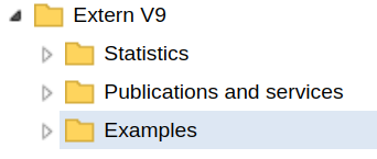
The first function shows the catalogue, which lists all available databases in a tree form. The tree structure is determined by the API and closely resembles the “Catalogue” view in the GUI.

my_catalogue <- sc_schema_catalogue()
my_catalogue

FOLDER: Extern V9
# A data frame: 6 × 3
  child                     type   n_childs
  <chr>                     <chr>     <int>
1 Examples                  FOLDER        9
2 Publications and services FOLDER        2
3 Default Tables            FOLDER        0
4 Statistics                FOLDER       20
5 meineErsteTabelle         TABLE         0
6 meineZweiteTabelle        TABLE         0

We see that the catalog has 8 child nodes: Four childs of type FOLDER and four childs of type TABLE. The table nodes correspond to the saved tables as described in the saved tables article. The folders include all folders from the root level in the catalogue explorer: “Statistics”, “Publication and Services” as well as “Examples”.

To get access to the child nodes use my_catalogue${child_label}

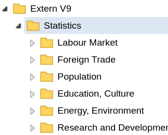
my_catalogue$Statistics

FOLDER: Statistics
# A data frame: 20 × 3
  child               type   n_childs
  <chr>               <chr>     <int>
1 Labour Market       FOLDER       15
2 Foreign Trade       FOLDER        4
3 Population          FOLDER       16
4 Education, Culture  FOLDER        5
5 Energy, Environment FOLDER        2
# ℹ 15 more rows

The child node Statistics is also of class sc_schema and shows all entries of the subfolder.

This syntax can be used to navigate through folders and subfolders.

my_catalogue$Statistics$`Foreign Trade`

FOLDER: Foreign Trade
# A data frame: 4 × 3
  child                                     type   n_childs
  <chr>                                     <chr>     <int>
1 TEC - Trade by enterprise characteristics FOLDER       20
2 Außenhandelsindizes                       FOLDER        0
3 Foreign Trade; Absolute Data              FOLDER       12
4 Regional data by federal provinces        FOLDER        6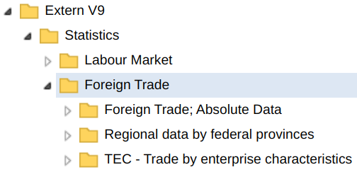

In some cases, the API shows more folders than the GUI in which case the folders from the API will be empty.

my_catalogue$Statistics$`Foreign Trade`$Außenhandelsindizes

FOLDER: Außenhandelsindizes

Databases and Tables

Inside the catalogue, the leafs¹ of the tree are mostly of type DATABASE and TABLE.

my_catalogue$Statistics$`Foreign Trade`$`Regional data by federal provinces`

FOLDER: Regional data by federal provinces
# A data frame: 6 × 3
  child                                                     type     n_childs
  <chr>                                                     <chr>       <int>
1 Regional data by federal provinces and 2digits CN         DATABASE        0
2 Regional data by federal provinces and countries          DATABASE        0
3 Regional data by federal provinces and country groups     DATABASE        0
4 Standardtabelle / Default table (defaulttable_deahbdllgr) TABLE           0
5 Standardtabelle / Default table (defaulttable_deahbdlld)  TABLE           0
# ℹ 1 more row

Here is an example for the DATABASE node deake005.

my_catalogue$Statistics$`Labour Market`$`Working hours (Labour Force Survey)`

DATABASE: Working hours (Labour Force Survey)
# Get more info with `STATcubeR::sc_schema_db('str:datab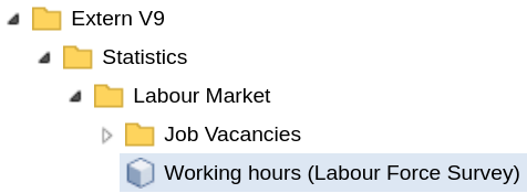ase:deake005')`

The function sc_schema_db() will be shown in the next section. As an example for a TABLE node, consider the default table for deake005.

my_catalogue$Statistics$`Labour Market`$
  `Standardtabelle / Default table (defaulttable_deake005)`

TABLE: Standardtabelle / Default table (defaulttable_deake005)
Get the data with `STATcubeR::sc_table_saved('str:table:defaulttable_deake005')`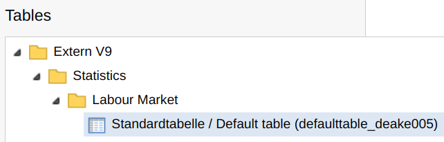

As suggested by the output, tables can be loaded with the /table endpoint via sc_table_saved(). See the saved tables article for more details.

Database Infos

To get information about a specific database, you can pass the database id to sc_schema_db(). Similar to sc_schema_catalogue(), the return value has a tree-like data structure.

my_db_info <- sc_schema_db("deake005")
my_db_info

DATABASE: Working hours (Labour Force Survey)
# A data frame: 8 × 3
  child                       type  n_childs
  <chr>                       <chr>    <int>
1 Factors                     GROUP        9
2 Datensätze/Records          GROUP        1
3 Time (mandatory field)      GROUP        1
4 Demographic Characteristics GROUP        8
5 Employment Characteristics  GROUP        6
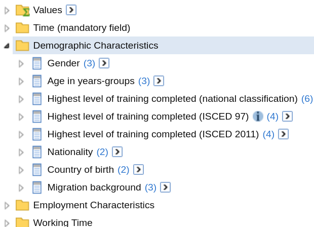
# ℹ 3 more rows

For comparison, here is a screenshot from the sidebar of the table view for deake005 which has a similar (but not identical) structure.

my_db_info can be used in a similar fashion as my_catalogue to obtain details about the resources in the tree. For example, the VALUESET with the label “Gender” can be viewed like this.

my_db_info$`Demographic Characteristics`

GROUP: Demographic Characteristics
# A data frame: 8 × 3
  child                                                         type  n_childs
  <chr>                                                         <chr>    <int>
1 Gender                                                        FIELD        1
2 Age in years-groups                                           FIELD        3
3 Highest level of training completed (national classification) FIELD        2
4 Highest level of training completed (ISCED 97)                FIELD        2
5 Highest level of training completed (ISCED 2011)              FIELD        2
# ℹ 3 more rows

my_db_info$`Demographic Characteristics`$Gender$Gender

VALUESET: Gender
# A data frame: 3 × 3
  child                type  n_childs
  <chr>                <chr>    <int>
1 male                 VALUE        0
2 female               VALUE        0
3 Not classifiable <0> VALUE        0

my_db_info$`Demographic Characteristics`$Gender$Gender$male

VALUE: male

The leafs of database schemas are mostly of type VALUE and MEASURE.

Data Structure of sc_schema Objects

As shown above, sc_schema objets have a tree like structure. Each sc_schema object has id, label, location and type as the last four entries

str(tail(my_db_info$`Demographic Characteristics`, 4))

#> List of 4
#>  $ id      : chr "str:group:deake005:X_B1"
#>  $ label   : chr "Demographic Characteristics"
#>  $ location: chr "http://statcubeapi.statistik.at/statistik.at/ext/statcube/rest/v1/schema/str:group:deake005:X_B1"
#>  $ type    : chr "GROUP"

str(tail(my_catalogue$Statistics, 4))

#> List of 4
#>  $ id      : chr "str:folder:festat"
#>  $ label   : chr "Statistics"
#>  $ location: chr "http://statcubeapi.statistik.at/statistik.at/ext/statcube/rest/v1/schema/str:folder:festat"
#>  $ type    : chr "FOLDER"

Schema objects can have an arbitrary amount of children. Children are always of type sc_schema. x$type contains the type of the schema object. A complete list of schema types is avilable in the API reference.

Other Resources

Information about resources other than databases and the catalogue can be obtained by passing the resource id to sc_schema().

(id <- my_db_info$Factors$id)
#> [1] "str:group:deake005:M_F1"
group_info <- sc_schema(id)
group_info

GROUP: Factors
# A data frame: 9 × 3
  child                                                         type    n_childs
  <chr>                                                         <chr>      <int>
1 Average hours actually worked per week                        MEASURE        0
2 Average hours usually worked per week                         MEASURE        0
3 Volume of hours worked in the main job per year in million h… MEASURE        0
4 Volume of hours worked overtime (paid) per year in million h… MEASURE        0
5 Volume of hours worked overtime (unpaid) per year in million… MEASURE        0
# ℹ 4 more rows

Note that the tree returned only has depth 1, i.e. the child nodes of measures are not available in group_info. However, ids of the child nodes can be obtained with $id. These ids can be used to send another request to the /schema endpoint

(id <- group_info$`Average hours usually worked per week`$id)
#> [1] "str:measure:deake005:F-DATA:F-FAKTOR2"
measure_info <- sc_schema(id)

Alternatively, use the depth parameter of sc_schema(). This will make sure that the entries of the tree are returned recursively up to a certain level. For example, depth = "VALUESET" will use the same level of recursion as sc_schema_db(). See ?sc_schema for all available options of the depth parameter.

group_info <- my_db_info$`Demographic Characteristics`$id %>%
  sc_schema(depth = "valueset")

Printing with data.tree

If the data.tree package is installed, it can be used for an alternative print mehtod.

print(group_info, tree = TRUE)

#>                           levelName     type
#> 1  Demographic Characteristics         GROUP
#> 2   ¦--Gender                          FIELD
#> 3   ¦   °--Gender                   VALUESET
#> 4   ¦       ¦--male                    VALUE
#> 5   ¦       ¦--female                  VALUE
#> 6   ¦       °--Not classifiable <0>    VALUE
#> 7   ¦--Age in years-groups             FIELD
#> 8   ¦   ¦--Age in years-groups      VALUESET
#> 9   ¦   ¦   ¦--Under 15 years          VALUE
#> 10  ¦   ¦   ¦--15 to 19 years          VALUE
#> 11  ¦   ¦   ¦--20 to 24 years          VALUE
#> 12  ¦   ¦   ¦--25 to 29 years          VALUE
#> 13  ¦   ¦   ¦--30 to 34 years          VALUE
#> 14  ¦   ¦   ¦--35 to 39 years          VALUE
#> 15  ¦   ¦   ¦--40 to 44 years          VALUE
#> 16  ¦   ¦   ¦--45 to 49 years          VALUE
#> 17  ¦   ¦   ¦--50 to 54 years          VALUE
#> 18  ¦   ¦   ¦--55 to 59 years          VALUE
#> 19  ¦   ¦   ¦--60 to 64 years          VALUE
#> 20  ¦   ¦   ¦--65 to 69 years          VALUE
#> 21  ¦   ¦   ¦--70 to 74 years          VALUE
#> 22  ¦   ¦   ¦--75 years and older      VALUE
#> 23  ¦   ¦   °--Not classifiable <0>    VALUE
#> 24  ¦   ¦--Alter in Jahresgruppen   VALUESET
#> 25  ¦   ¦   ¦--Under 15 years          VALUE
#> 26  ¦   ¦   ¦--15 to 24 years          VALUE
#> 27  ¦   ¦   ¦--25 to 34 years          VALUE
#> 28  ¦   ¦   ¦--35 to 44 years          VALUE
#> 29  ¦   ¦   ¦--45 to 54 years          VALUE
#> 30  ¦   ¦   °--... 3 nodes w/ 0 sub         
#> 31  ¦   °--... 1 nodes w/ 6 sub             
#> 32  °--... 6 nodes w/ 80 sub

The data.tree implementation of the print method can be set as a default using the option STATcubeR.print_tree

options(STATcubeR.print_tree = TRUE)

Flatten a Schema

The function sc_schema_flatten() can be used to turn responses from the /schema endpoint into data.frames. The following call extracts all databasess from the catalogue and displays their ids and labels.

sc_schema_catalogue() %>%
  sc_schema_flatten("DATABASE")

# A data frame: 641 × 2
  id                               label                 
  <chr>                            <chr>                 
1 str:database:dedemo              Communes (Demo)       
2 str:database:depeople            People                
3 str:database:depeopleml          People multilingual   
4 str:database:deretailml          Retail Banking ML en  
5 str:database:dekonjunkturmonitor Economic trend monitor
# ℹ 636 more rows

The string "DATABASE" in the previous example acts as a filter to make sure only nodes with the schema type DATABASE are included in the table.

If "DATABASE" is relaced with "TABLE", all tables will be displayed. This includes

All the defaulttables on STATcube. Most databases have an associated default table.
All saved tables for the current user as described in the saved tables article.
Other saved tables. Some databases do not only provide a default table but also several other tables. See this database on transport statistics as an example for database with more than one associated table

sc_schema_catalogue() %>%
  sc_schema_flatten("TABLE")

# A data frame: 674 × 2
  id                                             label                          
  <chr>                                          <chr>                          
1 str:table:7f851bfd-4bc0-4cc7-9013-e3c7982c9842 Monitoring                     
2 str:table:defaulttable_depeopleml              Standardtabelle / Default tabl…
3 str:table:defaulttable_dedemo                  Standardtabelle / Default tabl…
4 str:table:E-A_nach_Bundeslaendern_dedemo       E-A_nach_Bundeslaendern_dedemo 
5 str:table:Jahre_nach_NUTS_dedemo               Jahre_nach_NUTS_dedemo         
# ℹ 669 more rows

sc_schema_flatten() can also be used with sc_schema_db() and sc_schema(). The following example shows all available measures from the economic trend monitor database.

sc_schema_db("dekonjunkturmonitor") %>%
  sc_schema_flatten("MEASURE")

# A data frame: 88 × 2
  id                                              label                         
  <chr>                                           <chr>                         
1 str:measure:dekonjunkturmonitor:F-DATA:F-FAKT-1 Production index industry (wd…
2 str:measure:dekonjunkturmonitor:F-DATA:F-FAKT-2 Technical total production in…
3 str:measure:dekonjunkturmonitor:F-DATA:F-FAKT-3 Turnover index industry (2021…
4 str:measure:dekonjunkturmonitor:F-DATA:F-FAKT-4 Turnover industry (in 1.000 €)
5 str:measure:dekonjunkturmonitor:F-DATA:F-FAKT-5 Index of new orders industry …
# ℹ 83 more rows