Define Custom Tables

## ✔ Key could be verified via a test request

## ℹ The provided key will be available for this R session

## ℹ Add `STATCUBE_KEY_EXT = XXXX` to "~/.Renviron" to set the key
##   persistently. Replace `XXXX` with your key

The function sc_table_custom() allows you to define requests against the /table endpoint programmatically. This can be useful to automate the generation of /table request rather than relying on the GUI to do so. The function accepts the four arguments.

A database id
ids of measures to be imported (type MEASURE, STAT_FUNCTION or COUNT)
ids of fields to be imported (type FIELD or VALUESET)
a list of recodes that can be used customize fields

Building a Custom Table Step by Step

The first part of this Article will showcase how custom tables can be created with a database about tourism. This database will also be used in most other examples of this article.

Starting Simple

First, we want to just send the database id to sc_table_custom(). This will request only the mandatory fields and default measures for that database. In case of the tourism database, a table with one single row is returned.

database <- "str:database:detouextregsai"
x <- sc_table_custom(database)
x$tabulate()

# A STATcubeR tibble: 1 x 2
  `Season/Tourism Month` `Nights spent`
* <date>                          <dbl>
1 2024-06-01                   72541299

Show json request

x$json

 {
  "database": "str:database:detouextregsai",
  "measures": [],
  "dimensions": []
}

We see that 72 541 299 nights were spent in Austrian tourism establishments in the month of 2024-06-01.

Adding Countries

Now we want to add a classification to the table. This can be done by getting the database schema and showing all classification fields.

tourism <- sc_schema_db(database)
(fields <- sc_schema_flatten(tourism, "FIELD"))

# A data frame: 4 × 2
  id                                           label                     
  <chr>                                        <chr>                     
1 str:field:detouextregsai:F-DATA1:C-SDB_TIT-0 Season/Tourism Month      
2 str:field:detouextregsai:F-DATA:C-GEMREG-0   Tourism commune [ABO]     
3 str:field:detouextregsai:F-DATA:C-BBTR_REG-0 Accomodation establishment
4 str:field:detouextregsai:F-DATA1:C-C93-2     Country of origin

If we want to add “Country of origin” we need to include the fourth entry of the id column in our request.

x <- sc_table_custom(tourism, dimensions = fields$id[4])
x$tabulate()

# A STATcubeR tibble: 3 x 3
  `Season/Tourism Month` `Country of origin` `Nights spent`
* <date>                 <fct>                        <dbl>
1 2024-06-01             Austria                   20772909
2 2024-06-01             Germany                   28265099
3 2024-06-01             other countries           23503291

Show json request

x$json

 {
  "database": "str:database:detouextregsai",
  "measures": [],
  "dimensions": [
    ["str:field:detouextregsai:F-DATA1:C-C93-2"]
  ]
}

Alternatively, we could also pass the schema object for “country of origin”.

origin <- tourism$`Other Classifications`$`Country of origin`
x <- sc_table_custom(tourism, dimensions = origin)

Adding Tourism Communes

The dimensions parameter in sc_schema_custom() accepts vectors of field ids. Therefore, we can add the communes easily.

x <- sc_table_custom(tourism, dimensions = fields$id[c(2, 4)])
x$tabulate()

# A STATcubeR tibble: 321 x 4
   `Season/Tourism Month` `Tourism commune [ABO]`         `Country of origin`
 * <date>                 <fct>                           <fct>              
 1 2024-06-01             Achensee                        Austria            
 2 2024-06-01             Achensee                        Germany            
 3 2024-06-01             Achensee                        other countries    
 4 2024-06-01             Alpbachtal und Tiroler Seenland Austria            
 5 2024-06-01             Alpbachtal und Tiroler Seenland Germany            
 6 2024-06-01             Alpbachtal und Tiroler Seenland other countries    
 7 2024-06-01             Alpenregion Bludenz             Austria            
 8 2024-06-01             Alpenregion Bludenz             Germany            
 9 2024-06-01             Alpenregion Bludenz             other countries    
10 2024-06-01             Arlberg                         Austria            
# ℹ 311 more rows
# ℹ 1 more variable: `Nights spent` <dbl>

Show json request

x$json

 {
  "database": "str:database:detouextregsai",
  "measures": [],
  "dimensions": [
    ["str:field:detouextregsai:F-DATA:C-GEMREG-0"],
    ["str:field:detouextregsai:F-DATA1:C-C93-2"]
  ]
}

Add Another Measure

Currently, the table only returns the default measure for the database which is the number of nights spent. We can add a second measure by again using the database schema and passing a measure id

(measures <- sc_schema_flatten(tourism, "MEASURE"))

# A data frame: 2 × 2
  id                                       label       
  <chr>                                    <chr>       
1 str:measure:detouextregsai:F-DATA1:F-ANK Arrivals    
2 str:measure:detouextregsai:F-DATA1:F-UEB Nights spent

We can add both measures to the request by using measures$id. Just like the dimensions parameter, the measures parameters accepts vectors of resource ids.

x <- sc_table_custom(tourism, measures = measures$id,
                     dimensions = fields$id[c(2, 4)])
x$tabulate()

# A STATcubeR tibble: 321 x 5
   `Season/Tourism Month` `Tourism commune [ABO]`         `Country of origin`
 * <date>                 <fct>                           <fct>              
 1 2024-06-01             Achensee                        Austria            
 2 2024-06-01             Achensee                        Germany            
 3 2024-06-01             Achensee                        other countries    
 4 2024-06-01             Alpbachtal und Tiroler Seenland Austria            
 5 2024-06-01             Alpbachtal und Tiroler Seenland Germany            
 6 2024-06-01             Alpbachtal und Tiroler Seenland other countries    
 7 2024-06-01             Alpenregion Bludenz             Austria            
 8 2024-06-01             Alpenregion Bludenz             Germany            
 9 2024-06-01             Alpenregion Bludenz             other countries    
10 2024-06-01             Arlberg                         Austria            
# ℹ 311 more rows
# ℹ 2 more variables: Arrivals <dbl>, `Nights spent` <dbl>

Show json request

x$json

 {
  "database": "str:database:detouextregsai",
  "measures": [
    "str:measure:detouextregsai:F-DATA1:F-ANK",
    "str:measure:detouextregsai:F-DATA1:F-UEB"
  ],
  "dimensions": [
    ["str:field:detouextregsai:F-DATA:C-GEMREG-0"],
    ["str:field:detouextregsai:F-DATA1:C-C93-2"]
  ]
}

Changing the hierarchy level

We can see in the GUI that “Country of origin” is a hierarchical classification. If we look at the table above, only the top level of the hierarchy (Austria, Germany, other) is used. This can be changed by providing the the value-set that corresponds to the more granular classification of “country of origin”

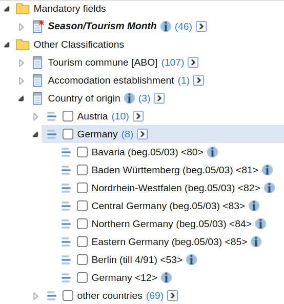
The different value-sets for “country of origin” can be compared by browsing the database schema.

(valuesets <- tourism$`Other Classifications`$`Country of origin`)

#> FIELD: Country of origin
#> 1 Country of origin        VALUESET    87
#> 2 Herkunftsland (Ebene +1) VALUESET     3

We can see that the two levels of the hierarchy are represented by the two value-sets. The value-set “Herkunftsland” uses 3 classification elements and represents the top level of the hierarchy (Austria, Germany, Other). The value-set “Country of origin” uses 87 (10+8+69) classification elements and is the bottom level of the hierarchy. For classifications with more levels of hierarchies, more value-sets will be present.

We will now use the id for the first value-set in the dimensions parameter of sc_table_custom.

x <- sc_table_custom(
  db = tourism,
  measures = measures$id,
  dimensions = valuesets$`Country of origin`
)
x$tabulate()

# A STATcubeR tibble: 87 x 4
   `Season/Tourism Month` `Country of origin`            Arrivals `Nights spent`
 * <date>                 <fct>                             <dbl>          <dbl>
 1 2024-06-01             Vienna <01>                     1573335        4611702
 2 2024-06-01             Burgenland (beg.05/03) <70>      380208         980905
 3 2024-06-01             Carinthia (beg.05/03) <71>       396573        1154423
 4 2024-06-01             Lower Austria (beg.05/03) <72>  1391481        4168398
 5 2024-06-01             Upper Austria (beg.05/03) <73>  1280137        3475584
 6 2024-06-01             Salzburg (beg.05/03) <74>        525320        1327853
 7 2024-06-01             Styria (beg.05/03) <75>         1030881        2973213
 8 2024-06-01             Tyrol (beg.05/03) <76>           536937        1371695
 9 2024-06-01             Vorarlberg (beg.05/03) <77>      274097         709136
10 2024-06-01             Austria except Vienna (till 0…        0              0
# ℹ 77 more rows

Show json request

x$json

 {
  "database": "str:database:detouextregsai",
  "measures": [
    "str:measure:detouextregsai:F-DATA1:F-ANK",
    "str:measure:detouextregsai:F-DATA1:F-UEB"
  ],
  "dimensions": [
    ["str:valueset:detouextregsai:F-DATA1:C-C93-2:C-C93-2"]
  ]
}

It is possible to use a mixture of value-sets and fields in the dimensions parameter.

Using Counts

Instead of Measures and Value-sets, it is also possible to provide counts in the measure parameter of sc_table_custom().

population <- sc_schema_db("debevstand")
(count <- population$`Datensätze/Records`$`F-BEVSTAND`)

#> COUNT: F-BEVSTAND

x <- sc_table_custom(population, count)
x$tabulate()

# A STATcubeR tibble: 1 x 2
  Quarter    `F-BEVSTAND`
* <date>            <dbl>
1 2024-01-01       389629

Show json request

x$json

 {
  "database": "str:database:debevstand",
  "measures": [
    "str:count:debevstand:F-BEVSTAND"
  ],
  "dimensions": []
}

Recodes

Data can be filtered on the server side by using the recodes parameter of sc_table_custom(). This might be more complicated than filtering the data in R but offers some important advantages.

performance Traffic between the client and server is reduced which might lead to considerably faster API responses.
cell limits (user) Apart from rate limits (see ?sc_rate_limits), STATcube also limits the amount of cells that can be fetched per user. Filtering data can be useful to preserve this quota.
cell limits (request) If a single request would contain more than 1 million cells, a cell count error is thrown.

Filtering Data

As an example for filtering data, we can request a table from the tourism database and only select some countries for Country of origin.

origin <- tourism$`Other Classifications`$`Country of origin`$`Country of origin`
month <- tourism$`Mandatory fields`$`Season/Tourism Month`$`Season/Tourism Month`
x <- sc_table_custom(
  db = tourism,
  measures = measures$id,
  dimensions = list(month, origin),
  recodes = sc_recode(origin, list(origin$`Italy <29>`, origin$`Germany <12>`))
)
x$tabulate()

# A STATcubeR tibble: 598 x 4
   `Season/Tourism Month` `Country of origin` Arrivals `Nights spent`
   <date>                 <fct>                  <dbl>          <dbl>
 1 1999-11-01             Italy <29>             34612          71854
 2 1999-11-01             Germany <12>          261213         762568
 3 1999-12-01             Italy <29>             88337         218213
 4 1999-12-01             Germany <12>          849720        4152811
 5 2000-01-01             Italy <29>             53289         204169
 6 2000-01-01             Germany <12>         1221916        6972223
 7 2000-02-01             Italy <29>             32509          98706
 8 2000-02-01             Germany <12>          966214        5651428
 9 2000-03-01             Italy <29>             56189         135877
10 2000-03-01             Germany <12>         1009715        5483191
# ℹ 588 more rows

Show json request

x$json

 {
  "database": "str:database:detouextregsai",
  "measures": [
    "str:measure:detouextregsai:F-DATA1:F-ANK",
    "str:measure:detouextregsai:F-DATA1:F-UEB"
  ],
  "dimensions": [
    ["str:valueset:detouextregsai:F-DATA1:C-SDB_TIT-0:C-SDB_TIT-0"],
    ["str:valueset:detouextregsai:F-DATA1:C-C93-2:C-C93-2"]
  ],
  "recodes": {
    "str:valueset:detouextregsai:F-DATA1:C-C93-2:C-C93-2": {
      "map": [
        ["str:value:detouextregsai:F-DATA1:C-C93-2:C-C93-2:20"],
        ["str:value:detouextregsai:F-DATA1:C-C93-2:C-C93-2:12"]
      ],
      "total": false
    }
  }
}

This table only contains two countries rather than 87 so the amount of cells in the table is also 40 times less compared to a table that would omit this filter.

Grouping items

Other options from the recodes specification are also available via sc_recode(). It is possible to group items and specify recodes for several classifications.

x <- sc_table_custom(
  db = tourism,
  measures = measures$id,
  dimensions = list(month, origin),
  recodes = c(
    sc_recode(origin, list(
      list(origin$`Germany <12>`, origin$`Netherlands <25>`),
      list(origin$`Italy <29>`, origin$`France (incl.Monaco) <14>`)
    )),
    sc_recode(month, list(
      month$Nov.99, month$Feb.00, month$Apr.09, month$`Jan. 22`
    ))
  )
)
x$tabulate()

# A STATcubeR tibble: 8 x 4
  `Season/Tourism Month` `Country of origin`             Arrivals `Nights spent`
  <date>                 <fct>                              <dbl>          <dbl>
1 1999-11-01             Germany <12>;Netherlands <25>     272496         795183
2 1999-11-01             Italy <29>;France (incl.Monaco…    47580         105150
3 2000-02-01             Germany <12>;Netherlands <25>    1237039        7208626
4 2000-02-01             Italy <29>;France (incl.Monaco…    77162         350655
5 2009-04-01             Germany <12>;Netherlands <25>      44545         174388
6 2009-04-01             Italy <29>;France (incl.Monaco…    97913         219553
7 2022-01-01             Germany <12>;Netherlands <25>     154121         886490
8 2022-01-01             Italy <29>;France (incl.Monaco…    28301         100484

Show json request

x$json

 {
  "database": "str:database:detouextregsai",
  "measures": [
    "str:measure:detouextregsai:F-DATA1:F-ANK",
    "str:measure:detouextregsai:F-DATA1:F-UEB"
  ],
  "dimensions": [
    ["str:valueset:detouextregsai:F-DATA1:C-SDB_TIT-0:C-SDB_TIT-0"],
    ["str:valueset:detouextregsai:F-DATA1:C-C93-2:C-C93-2"]
  ],
  "recodes": {
    "str:valueset:detouextregsai:F-DATA1:C-C93-2:C-C93-2": {
      "map": [
        ["str:value:detouextregsai:F-DATA1:C-C93-2:C-C93-2:12", "str:value:detouextregsai:F-DATA1:C-C93-2:C-C93-2:25"],
        ["str:value:detouextregsai:F-DATA1:C-C93-2:C-C93-2:20", "str:value:detouextregsai:F-DATA1:C-C93-2:C-C93-2:14"]
      ],
      "total": false
    },
    "str:valueset:detouextregsai:F-DATA1:C-SDB_TIT-0:C-SDB_TIT-0": {
      "map": [
        ["str:value:detouextregsai:F-DATA1:C-SDB_TIT-0:C-SDB_TIT-0:199911"],
        ["str:value:detouextregsai:F-DATA1:C-SDB_TIT-0:C-SDB_TIT-0:200002"],
        ["str:value:detouextregsai:F-DATA1:C-SDB_TIT-0:C-SDB_TIT-0:200904"],
        ["str:value:detouextregsai:F-DATA1:C-SDB_TIT-0:C-SDB_TIT-0:202201"]
      ],
      "total": false
    }
  }
}

This table contains data for two country-groups and two months. In this case, the cell values for Germany and the Netherlands are just added to calculate the entries for Arrivals and Nights spent. However, in other cases STATcube might decide it is more appropriate to use weighted means or other more complicated aggregation methods.

Adding Totals

The total parameter in sc_recode() can be used to request totals for classifications. As an example, let’s look at the tourism activity in the capital cities of Austria

destination <- tourism$`Other Classifications`$`Tourism commune [ABO]`$
  `Regionale Gliederung (Ebene +1)`
x <- sc_table_custom(
    tourism,
    measures = measures$id,
    dimensions = list(month, destination),
    recodes = c(
      sc_recode(destination, total = TRUE, list(
        destination$Wien, destination$`Stadt Salzburg`, destination$Linz)),
      sc_recode(month, total = FALSE, list(month$Nov.99, month$Apr.09))
    )
)
as.data.frame(x)

# A STATcubeR tibble: 8 x 4
  `Season/Tourism Month` `Tourism commune [ABO]` Arrivals `Nights spent`
  <date>                 <fct>                      <dbl>          <dbl>
1 1999-11-01             Wien                      234186         522306
2 1999-11-01             Stadt Salzburg             49369          89637
3 1999-11-01             Linz                       25562          43789
4 1999-11-01             Total                     309117         655732
5 2009-04-01             Wien                      356723         806201
6 2009-04-01             Stadt Salzburg             84582         151483
7 2009-04-01             Linz                       35594          65001
8 2009-04-01             Total                     476899        1022685

Show json request

x$json

 {
  "database": "str:database:detouextregsai",
  "measures": [
    "str:measure:detouextregsai:F-DATA1:F-ANK",
    "str:measure:detouextregsai:F-DATA1:F-UEB"
  ],
  "dimensions": [
    ["str:valueset:detouextregsai:F-DATA1:C-SDB_TIT-0:C-SDB_TIT-0"],
    ["str:valueset:detouextregsai:F-DATA:C-GEMREG-0:C-TOUREG-0"]
  ],
  "recodes": {
    "str:valueset:detouextregsai:F-DATA:C-GEMREG-0:C-TOUREG-0": {
      "map": [
        ["str:value:detouextregsai:F-DATA:C-GEMREG-0:C-TOUREG-0:TOUREG-Wien"],
        ["str:value:detouextregsai:F-DATA:C-GEMREG-0:C-TOUREG-0:TOUREG-Stadt"],
        ["str:value:detouextregsai:F-DATA:C-GEMREG-0:C-TOUREG-0:TOUREG-Linz"]
      ],
      "total": true
    },
    "str:valueset:detouextregsai:F-DATA1:C-SDB_TIT-0:C-SDB_TIT-0": {
      "map": [
        ["str:value:detouextregsai:F-DATA1:C-SDB_TIT-0:C-SDB_TIT-0:199911"],
        ["str:value:detouextregsai:F-DATA1:C-SDB_TIT-0:C-SDB_TIT-0:200904"]
      ],
      "total": false
    }
  }
}

We see that there are two rows in the table where Tourism commune is set to “Total”. The corresponding values represent the sum of all Arrivals or Nights spent in either of these three cities during that month.

Recoding across hierarchies

To use a recode that includes several hierarchy levels, the corresponding FIELD should be used as the first parameter of sc_recode(). For example, a recode with countries and federal states from the “Country of origin” classification can be defined as follows.

origin1 <- tourism$`Other Classifications`$`Country of origin`
origin2 <- origin1$`Country of origin`
origin3 <- origin1$`Herkunftsland (Ebene +1)`
x <- sc_table_custom(
  tourism, measures$id, origin1,
  recodes = sc_recode(origin1, list(
    origin2$`Vienna <01>`, origin3$Germany,
    list(origin2$`Bavaria (beg.05/03) <80>`, origin3$`other countries`))
  )
)
x$tabulate()

# A STATcubeR tibble: 3 x 4
  `Season/Tourism Month` `Country of origin`             Arrivals `Nights spent`
* <date>                 <fct>                              <dbl>          <dbl>
1 2024-06-01             Vienna <01>                      1573335        4611702
2 2024-06-01             Germany                          7562533       28265099
3 2024-06-01             other countries;Bavaria (beg.0… 10613351       30861772

Show json request

x$json

 {
  "database": "str:database:detouextregsai",
  "measures": [
    "str:measure:detouextregsai:F-DATA1:F-ANK",
    "str:measure:detouextregsai:F-DATA1:F-UEB"
  ],
  "dimensions": [
    ["str:field:detouextregsai:F-DATA1:C-C93-2"]
  ],
  "recodes": {
    "str:field:detouextregsai:F-DATA1:C-C93-2": {
      "map": [
        ["str:value:detouextregsai:F-DATA1:C-C93-2:C-C93-2:01"],
        ["str:value:detouextregsai:F-DATA1:C-C93-2:C-C93SUM-0:C93SUM-2"],
        ["str:value:detouextregsai:F-DATA1:C-C93-2:C-C93-2:80", "str:value:detouextregsai:F-DATA1:C-C93-2:C-C93SUM-0:C93SUM-3"]
      ],
      "total": false
    }
  }
}

Typechecks

Since custom tables can become quite complicated, sc_table_custom() performs type-checks before sending the request to the API. If inconsistencies are detected, warnings will be generated. See ?sc_table_custom for a comprehensive list of the performed checks.

sc_table_custom(tourism, measures = tourism, dry_run = TRUE)

#> Warning in sc_table_custom(tourism, measures = tourism, dry_run = TRUE):
#> parameter `measures` is not of type `MEASURE`, `STATFN` or `COUNT`

#> {
#>   "database": "str:database:detouextregsai",
#>   "measures": [
#>     "str:database:detouextregsai"
#>   ],
#>   "dimensions": []
#> }

Advanced example

sc_table_custom("A", measures = "B", dimensions = "C", 
                recodes = sc_recode("D", "E"), dry_run = TRUE)

#> Warning in sc_recode("D", "E"): parameters `field` and `map` might be
#> inconsistent

#> Warning in sc_recode("D", "E"): some entries in `map` are not of type VALUE

#> Warning in sc_recode("D", "E"): parameter `field` is not of type `FIELD` or
#> `VALUESET`

#> Warning in sc_table_custom("A", measures = "B", dimensions = "C", recodes =
#> sc_recode("D", : `recodes` and `dimensions` might be inconsistent

#> Warning in sc_table_custom("A", measures = "B", dimensions = "C", recodes =
#> sc_recode("D", : parameter `dimensions` is not of type `FIELD` or `VALUESET`

#> Warning in sc_table_custom("A", measures = "B", dimensions = "C", recodes =
#> sc_recode("D", : parameter `measures` is not of type `MEASURE`, `STATFN` or
#> `COUNT`

#> Warning in sc_table_custom("A", measures = "B", dimensions = "C", recodes =
#> sc_recode("D", : parameter `db` is not of type `DATABASE`

#> {
#>   "database": "A",
#>   "measures": [
#>     "B"
#>   ],
#>   "dimensions": [
#>     ["C"]
#>   ],
#>   "recodes": {
#>     "D": {
#>       "map": [
#>         ["E"]
#>       ],
#>       "total": false
#>     }
#>   }
#> }

If dry_run is set to FALSE (the default), STATcubeR will send the request to the API even if inconsistencies are detected. This will likely lead to an error of the form “expected json but got html”.

If you get spurious warnings or have suggestions on how these type-checks might be improved, please issue a feature request to the [STATcubeR bug tracker].

Building a Custom Table Step by Step

Starting Simple

Adding Countries

Adding Tourism Communes

Add Another Measure

Changing the hierarchy level

Using Counts

Recodes

Filtering Data

Grouping items

Adding Totals

Recoding across hierarchies

Typechecks

Further Reading