Introduction
This vignette demonstrates how to use the vimpute()
function for flexible missing data imputation using machine learning
models from the mlr3 ecosystem.
Function Arguments
-
data: A datatable or dataframe containing missing values to be imputed. -
considered_variables: A character vector of variable names to be either imputed or used as predictors, excluding irrelevant columns from the imputation process. -
method: A named list specifying the imputation method for each variable. If not set explicitly,vimpute()uses"ranger"for all considered variables. -
pmm: TRUE/FALSE indicating whether predictive mean matching is used. -
pmm_k: Number of nearest neighbors used for PMM. -
pmm_k_method: Strategy for selecting PMM donor values from theknearest candidates. -
learner_params: Optional learner-specific parameter lists for each variable (e.g.rangersettings such asmedian = TRUE). -
formula: If not all variables are used as predictors, or if transformations or interactions are required (applies to all X, for Y only transformations are possible). Only applicable for the methods"robust","regularized","gam"and"robgam". Provide as a list for each variable that requires specific conditions. -
makeNA: Optional named list of values that should be treated as imputable missing values for selected variables. -
donorcond: Optional named list of donor conditions used to restrict the observed training values for selected variables. -
sequential: Specifies whether the imputation should be performed sequentially. -
nseq: The number of sequential iterations, ifsequentialis TRUE. -
eps: The convergence threshold for sequential imputation. -
imp_var: Specifies whether to add indicator variables for imputed values. -
pred_history: If enabled, saves the prediction history. -
tune: Whether to perform hyperparameter tuning. -
verbose: If enabled, prints additional debugging output. -
boot: Whether to refit models on bootstrap samples to add model uncertainty. -
robustboot: Bootstrap sampling strategy used whenboot = TRUE. -
uncert: Prediction uncertainty method ("none","normalerror","resid","pmm","midastouch"). -
m: Number of multiple imputations. Ifm > 1, avimmiobject is returned.
Data
To demonstrate the function, the sleep dataset from the
VIM package is used.
data <- as.data.table(VIM::sleep)
a <- aggr(sleep, plot = FALSE)
plot(a, numbers = TRUE, prop = FALSE)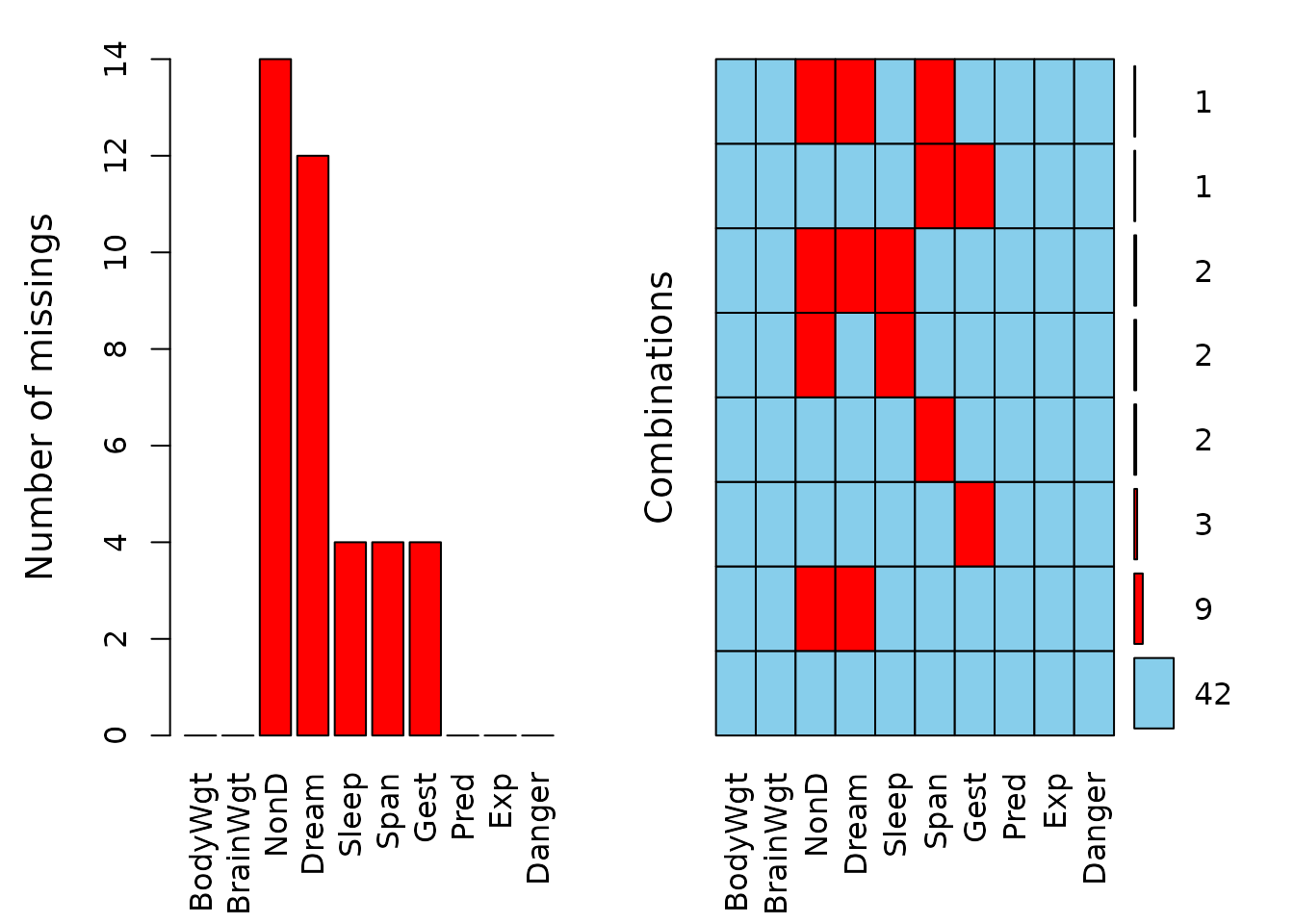
The left plot shows the amount of missings for each column in the dataset sleep and the right plot shows how often each combination of missings occur. For example, there are 9 rows wich contain a missing in both NonD and Dream.
dataDS <- sleep[, c("Dream", "Sleep")]
marginplot(dataDS, main = "Missing Values")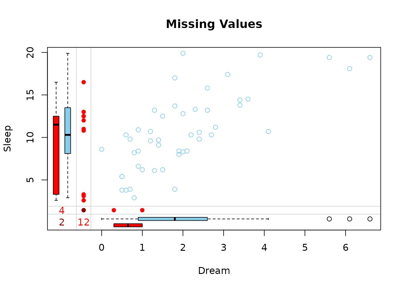
The red boxplot on the left shows the distrubution of all values of Sleep where Dream contains a missing value. The blue boxplot on the left shows the distribution of the values of Sleep where Dream is observed.
Basic Usage
Default Imputation
In the basic usage, the vimpute() function uses the
default settings: all variables are imputed with the “ranger” method,
sequential imputation is enabled (nseq = 10,
eps = 0.005), PMM is off, formulas are off, no tuning is
performed, and imputation indicators are added.
result <- vimpute(
  data = data,
  pred_history = TRUE)
print(head(result$data, 3))
#>     BodyWgt BrainWgt  NonD Dream Sleep  Span  Gest  Pred   Exp Danger NonD_imp
#>       <num>    <num> <num> <num> <num> <num> <num> <num> <num>  <num>   <lgcl>
#> 1: 6654.000   5712.0   3.5   1.3   3.3  38.6   645     3     5      3     TRUE
#> 2:    1.000      6.6   6.3   2.0   8.3   4.5    42     3     1      3    FALSE
#> 3:    3.385     44.5  10.7   2.3  12.5  14.0    60     1     1      1     TRUE
#>    Dream_imp Sleep_imp Span_imp Gest_imp
#>       <lgcl>    <lgcl>   <lgcl>   <lgcl>
#> 1:      TRUE     FALSE    FALSE    FALSE
#> 2:     FALSE     FALSE    FALSE    FALSE
#> 3:      TRUE     FALSE    FALSE    FALSE
Results and information about missing/imputed values can be shown in the plot margins:
dataDS <- as.data.frame(result$data[, c("Dream", "Sleep", "Dream_imp", "Sleep_imp")])
marginplot(dataDS, delimiter = "_imp", main = "Imputation with Default Model")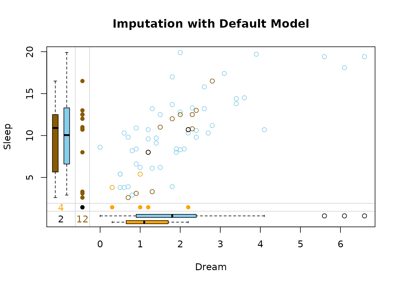
The default output are the imputed dataset and the prediction history.
In this plot three differnt colors are used in the top-right. These colors represent the structure of missings.
-
brown points represent
values where
Dreamwas missing initially -
beige points represent
values where
Sleepwas missing initially -
black points represent values where both
DreamandSleepwere missing initially
Advanced Options
Parameter method
(default: “ranger” for all variables)
Specifies the method used for imputation of each variable. If
method is not provided, vimpute() uses
"ranger" for all variables. In this example, different
imputation methods are specified for each variable. The
NonD variable uses a robust method, Dream and
Span are using ranger, Sleep uses xgboost,
Gest uses a regularized method and class uses
a robust method.
-
"robust": Robust Regression Models-
lmrobfor numeric variables: Implements MM-estimation for resistance to outliers -
glmrobfor factors: Robust GLM; binary via robust logit, multiclass via one-vs-rest
-
-
"regularized": Regularized Regression (glmnet)- Uses elastic net regularization
- Automatically handles multicollinearity
- Uses elastic net regularization
-
"ranger": Random Forest- Fast implementation of random forests
- Handles non-linear relationships well
- Fast implementation of random forests
-
"xgboost": Gradient Boosted Trees- State-of-the-art tree boosting
- Handles mixed data types well
- State-of-the-art tree boosting
-
"gam": Generalized Additive Models (mgcv)- Supports smooth terms for numeric predictors
- Can be used for numeric and factor targets
-
"robgam": Robust GAM- Adds robust weighting / refitting to GAM-style models
- Designed for settings with potential outliers
You can provide method globally as a single method name
(applies to all variables), or as a named list per variable.
result_mixed <- vimpute(
  data = data,
  method = list(NonD = "robust",
                Dream = "ranger",
                Sleep = "xgboost",
                Span = "ranger",
                Gest = "regularized"),
  pred_history = TRUE
  )
dataDS <- as.data.frame(result_mixed$data[, c("Dream", "Sleep", "Dream_imp", "Sleep_imp")])
marginplot(dataDS, delimiter = "_imp", main = "Imputation with different Models for each Variable")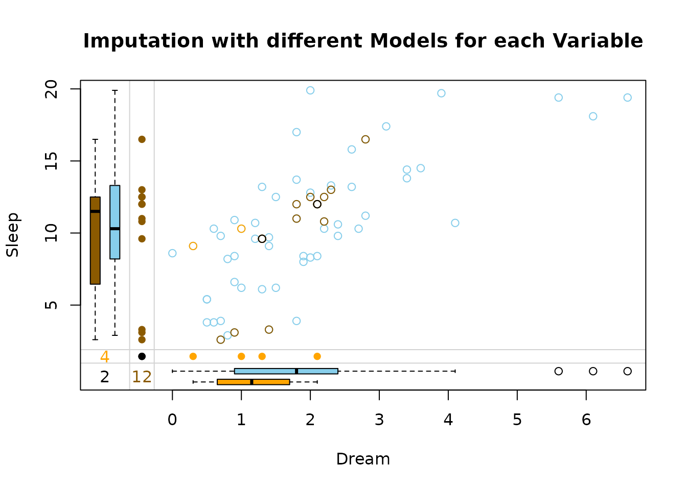
The side-by-side margin plots compare the performance of two imputation methods: xgboost (left) and regularized (right):
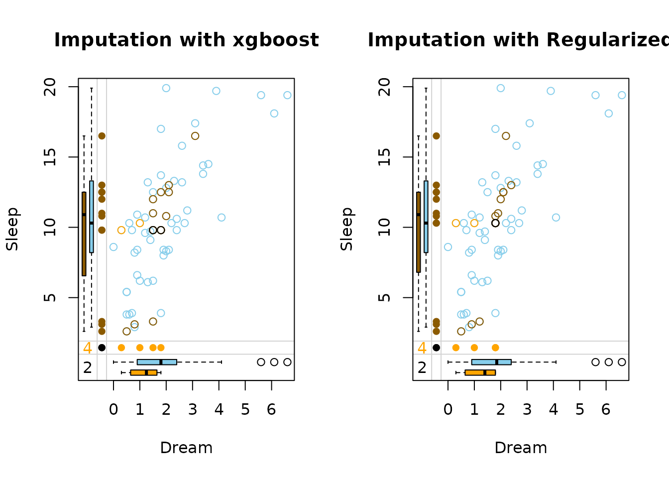
xgboost handles missing values with data-driven, uneven imputations that capture complex patterns but may be less stable, while regularized methods produce smoother, more conservative estimates that are less prone to overfitting. The key difference lies in flexibility (xgboost) versus robustness (regularization).
Parameter pmm
(default: FALSE)
result <- vimpute(
  data = data,
  method = list(NonD = "robust",
                Dream = "ranger",
                Sleep = "xgboost",
                Span = "ranger",
                Gest = "regularized"),
  pmm = list(NonD = FALSE, Dream = TRUE, Sleep = FALSE, Span = FALSE , Gest = TRUE)
  )
If pmm = TRUE, this is applied only to numeric target
variables.vimpute() first computes the model prediction for a missing
entry, then compares it to observed values of that target and selects
donor candidates by smallest absolute distance to the prediction.
If pmm_k = 1 (or NULL, which defaults to 1
when PMM is active), the closest observed value is used directly.
If pmm_k > 1, the final imputed value is derived from
the k nearest donors using pmm_k_method
(e.g. "mean", "median", "random"
or a custom function).
If pmm = FALSE, raw model predictions are used.
In sequential imputation, the convergence criterion is computed from the raw model prediction when PMM is active. This avoids unstable stopping behavior caused by stochastic or donor-based PMM values while still returning the PMM-imputed values in the final data.
You can provide pmm globally as a single logical value
(applies to all numeric variables), or as a named list per variable.
Parameter pmm_k
(default: NULL)
pmm_k defines how many nearest donor candidates are
considered when PMM is enabled.
You can provide pmm_k globally as a single integer value
(applies to all variables where PMM is active), or as a named list per
variable.
Parameter pmm_k_method
(default: “mean”)
pmm_k_method controls how the final donor value is
derived when pmm_k > 1. Possible values are:
-
"mean"(default): uses the mean of theknearest observed donor candidates. -
"median": uses the median of theknearest donor candidates (more robust to outliers). -
"random": randomly draws one value from theknearest donor candidates. -
"custom function": a function that gets theknearest donor values and returns one numeric value.
If a variable-specific list contains NULL,
vimpute() falls back to "mean" for that
variable.
You can provide pmm_k_method globally as a single
value/function (applies to all numeric variables where
pmm = TRUE and pmm_k > 1), or as a named
list per variable.
result <- vimpute(
  data = data,
  pmm = list(Dream = TRUE, Sleep = TRUE, NonD = FALSE),
  pmm_k = list(Dream = 5, Sleep = 3),
  pmm_k_method = list(
    Dream = "median",
    Sleep = "random"
  )
)
Custom aggregation functions are also possible. The function receives the nearest donor values and must return exactly one non-missing numeric value.
Parameter learner_params
(default: NULL)
Use learner_params to pass method-specific settings to
the underlying learners.
This is useful if different variables are imputed with different methods
and each method should receive its own parameter configuration.
You can provide learner_params globally (when one method
is used for all variables), as a method-level list, or as a named list
per variable.
Parameter formula
(default: FALSE)
Specifies custom model formulas for imputation of each variable, offering precise control over the imputation models.
Key Features:
-
Variable-Specific Models
Each formula specifies which predictors should be used for imputing a particular variable
Enables different predictor sets for different target variables
-
Example:
formula = list(
  income ~ education + age,
  blood_pressure ~ weight + age
)
-
Transformations Support
-
Handles common transformations on both sides of the formula:
- Response transformations:
log(y),sqrt(y),exp(y),I(1/y) - Predictor transformations:
log(x1),poly(x2, 2), etc.
- Response transformations:
-
Example with transformations:
-
-
Interaction Terms
Supports interaction terms using
:or*syntax (on the right side)-
Example:
formula = list(
  price ~ sqft * neighborhood + year_built
)
Example Demonstration:
result <- vimpute(
  data = data,
  method = setNames(as.list(rep("regularized", ncol(data))), names(data)),
  formula = list(
    NonD ~ Dream + Sleep,              # Linear combination
    Span ~ Dream:Sleep + Gest,         # With interaction term
    log(Gest) ~ Sleep + exp(Span)      # With transformations
  )
)
Interpreting the Example:
- For
NonD:- Uses linear combination of
DreamandSleepvariables - Model:
NonD = β₀ + β₁*Dream + β₂*Sleep + ε
- Uses linear combination of
- For
Span:- Includes interaction between
DreamandSleep - Plus main effect of
Gest - Model:
Span = β₀ + β₁*Dream*Sleep + β₂*Gest + ε
- Includes interaction between
- For
Gest:- Uses log-transformed response
- Predictors include
Sleepand exponential ofSpan - Model:
log(Gest) = β₀ + β₁*Sleep + β₂*exp(Span) + ε
- For
SleepandDreamall other variables are used as predictors
Notes:
- Only works with methods
"robust","regularized","gam"and"robgam" - All model.matrix-compatible functions work for predictors (for more information see ?model.matrix)
- Response transformations (left side) are automatically back-transformed
Parameter makeNA
(default: NULL)
makeNA defines values that should be treated as missing
for selected variables. This is useful when special codes such as
-999, "unknown" or "not measured"
should be imputed, while regular NA values in the same
variable should remain untouched.
If a variable is listed in makeNA, only the matching
values are imputed for that variable. Variables not listed in
makeNA continue to use regular NA values as
the imputation target.
Parameter donorcond
(default: NULL)
donorcond restricts which observed values are allowed to
act as donors / training observations for a target variable. Conditions
are supplied as character strings and evaluated on the target values via
the temporary variable x.
result <- vimpute(
  data = data,
  method = list(Dream = "ranger"),
  donorcond = list(Dream = "> quantile(x, 0.1, na.rm = TRUE)")
)
This can be useful when implausible observed values should not be used for model fitting, while the target variable itself remains part of the imputation workflow.
Parameters boot, robustboot and
uncert
(defaults: boot = FALSE,
robustboot = "stratified",
uncert = "none")
These arguments control additional imputation uncertainty.
-
boot = TRUErefits the imputation model on a bootstrap sample. -
robustbootcontrols how bootstrap rows are sampled ("standard","stratified"or"residual"). -
uncertadds uncertainty to numeric predictions:-
"normalerror"adds normal noise using the model scale estimate. -
"resid"adds sampled residuals. -
"pmm"uses score-based predictive mean matching. -
"midastouch"uses PMM with covariate-distance weighting.
-
result <- vimpute(
  data = data,
  method = list(Dream = "ranger"),
  boot = TRUE,
  robustboot = "standard",
  uncert = "normalerror"
)
If explicit pmm = TRUE is used for a variable, it takes
precedence over uncert.
Parameter m
(default: 1)
m controls multiple imputation. If
m > 1, vimpute() returns a
vimmi object instead of a single completed dataset.
mi <- vimpute(
  data = data,
  method = list(Dream = "ranger"),
  m = 5,
  boot = TRUE,
  uncert = "resid",
  imp_var = FALSE
)

completed_1 <- complete(mi, 1)
completed_all <- complete(mi, "all")
completed_long <- complete(mi, "long")
The vimmi object stores the original data and the
imputed values efficiently. It can be inspected with
print() and summary(), and completed datasets
can be extracted with complete(). If the mice
package is installed, as.mids.vimmi() can be used to
convert a vimmi object to a mice::mids object
for downstream pooling workflows.
Parameter tune
(default: FALSE)
result <- vimpute(
  data = data,
  tune = TRUE
  )
Whether to perform hyperparameter tuning (only possible if seq = TRUE):
- When TRUE:
- Conducts randomized parameter search (after half of the iterations)
- Uses best performing configuration
- When FALSE:
- Uses default model parameters
- Recommended: TRUE for optimal performance
You can provide tune either as a single global
TRUE/FALSE value (applies to all variables), or as a named list per
variable.
When tuning is enabled, vimpute() returns a list
containing the imputed data and a tuning_log component. If
pred_history = TRUE is also enabled, the list contains both
pred_history and tuning_log.
Parameters nseq and eps
(default: 10 and default: 0.005)
result <- vimpute(
  data = data,
  nseq = 20,
  eps = 0.01
  )
nseq describes the number of sequential imputation
iterations. Higher values:
- Allow more refinement
- Increase computation time
eps describes the convergence threshold for sequential
imputation:
- Stops early if changes between iterations < eps
- Smaller values: Require more precise convergence but may need more iterations
Parameter imp_var
(default: TRUE)
result <- vimpute(
  data = data,
  imp_var = TRUE
  )
Creating indicator variables for imputed values adds “_imp” columns (TRUE/FALSE) to mark which data points were imputed. This is particularly useful for tracking imputation effects and conducting diagnostic analyses.
Parameter pred_history
(default: FALSE)
print(tail(result$pred_history, 9))
#>    iteration variable index predicted_values
#>        <int>   <char> <int>            <num>
#> 1:        10    Sleep    62             10.6
#> 2:        10     Span     4              6.9
#> 3:        10     Span    13              4.9
#> 4:        10     Span    35              5.0
#> 5:        10     Span    36              7.1
#> 6:        10     Gest    13             41.3
#> 7:        10     Gest    19            219.2
#> 8:        10     Gest    20             90.4
#> 9:        10     Gest    56             31.7
When enabled (TRUE), this option saves prediction trajectories in
$pred_history, allowing users to track how imputed values
evolve across iterations. This feature is particularly useful for
diagnosing convergence issues.
With pred_history = TRUE, vimpute() returns
a list (not only the imputed data table). Therefore, results must be
accessed via list elements, e.g. result$data for the
imputed dataset and result$pred_history for the
history.
Performance
In order to validate the performance of vimpute() the iris dataset is
used. Firstly, some values are randomly set to NA.
library(reactable)

data(iris)
df <- as.data.table(iris)
colnames(df) <- c("S.Length","S.Width","P.Length","P.Width","Species")
# randomly produce some missing values in the data
set.seed(1)
nbr_missing <- 50
y <- data.frame(row=sample(nrow(iris),size = nbr_missing,replace = T),
                col=sample(ncol(iris)-1,size = nbr_missing,replace = T))
y<-y[!duplicated(y),]
df[as.matrix(y)]<-NA

aggr(df)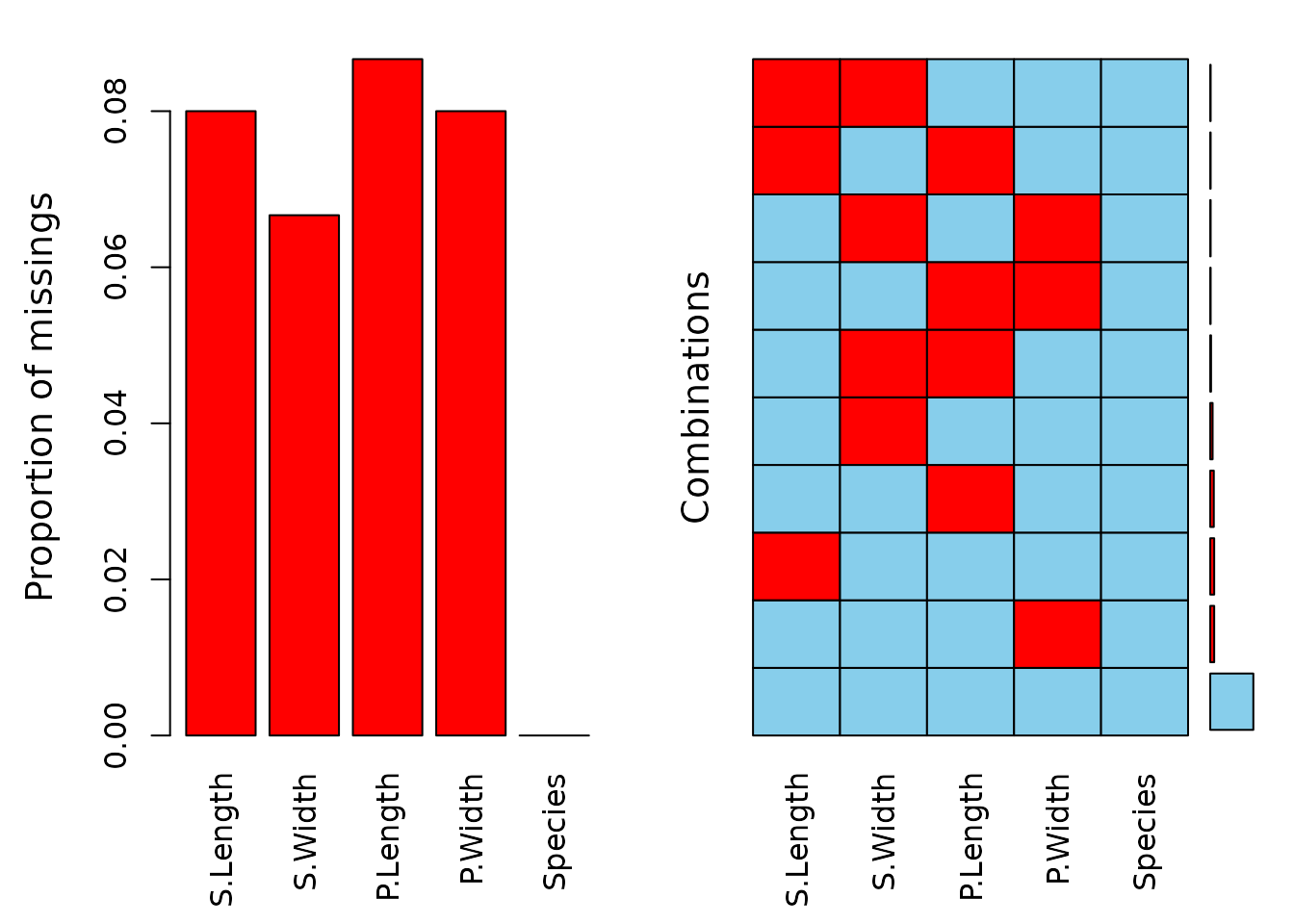
The data contains missing values across all variables, with some observations missing multiple values. The subsequent step involves variable imputation, and the following tables present the rounded first five imputation results for each variable.
For default model:
For xgboost model: