VIM

VIM introduces tools for visualization of missing and imputed values. Forthermore, methods to impute missing values are featured. This vignette will give a brief look at a common imputation scenario and showcase how VIM can be used to both impute the data and also interpret the results visually.

Visualize missing values

library(VIM)
data(sleep)
a <- aggr(sleep, plot = FALSE)
plot(a, numbers = TRUE, prop = FALSE)

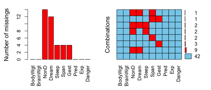
The left plot shows the amount of missings for each column in the dataset sleep and the right plot shows how often each combination of missings occur. For example, there are 9 rows wich contain a missing in both NonD and Dream.

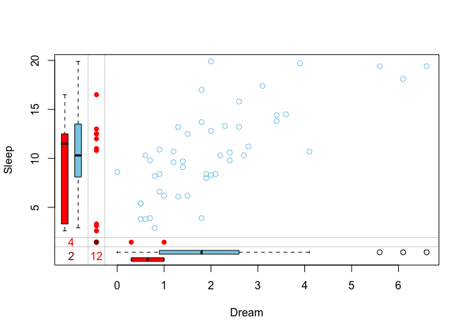
For simplicity, we will only look at the variables Dream and Sleep for the remainer of this vignette. Bivariate datasets can be passed to special functions that visualize the structure of missings such as marginplot().

x <- sleep[, c("Dream", "Sleep")]
marginplot(x)

The red boxplot on the left shows the distrubution of all values of Sleep where Dream contains a missing value. The blue boxplot on the left shows the distribution of the values of Sleep where Dream is observed.

Impute missing values

In order to impute missing values, VIM offers a spectrum of imputation methods like kNN() (k nearest neighbour), hotdeck() and so forth. Those functions can be applied to a data.frame and return another data.frame where missings are replaced by imputed values.

x_imputed <- kNN(x)

To learn more about all implemented imputation methods, three vignettes are available

• vignette("donorImp") explains the donor-based imputation methods hotdeck() and kNN()
• vignette("modelImp") gives insight into the model-based imputation methods regressionImp() and matchImpute()
• vignette("irmi") showcases the irmi() method.

Visualize imputed values

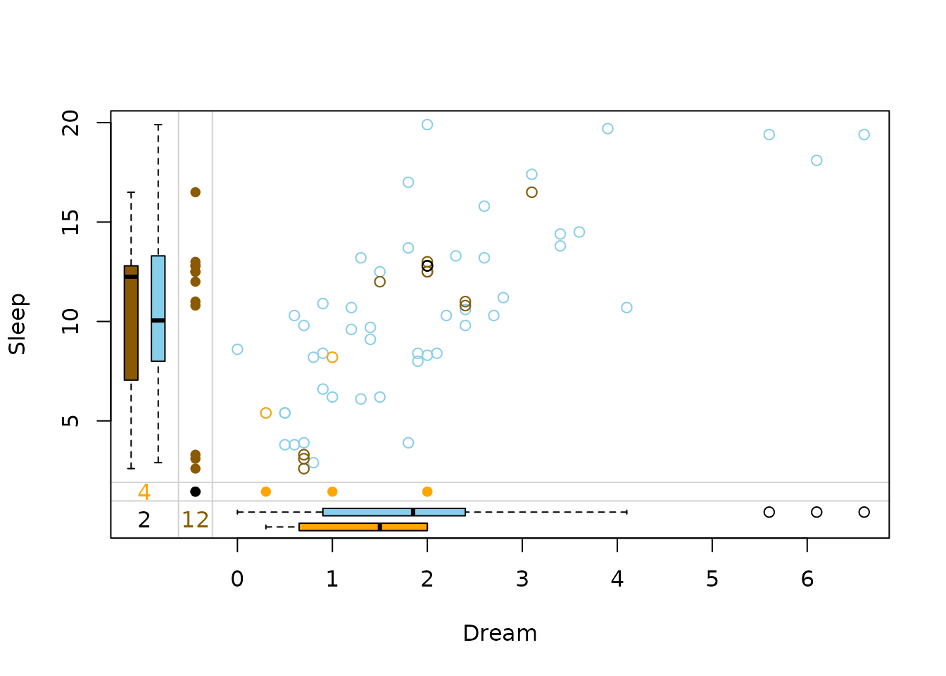
The same functions that visualize missing values can also visualize the imputed dataset.

marginplot(x_imputed, delimiter = "_imp")

In this plot three differnt colors are used in the top-right. These colors represent the structure of missings.

• brown points represent values where Dream was missing initially
• beige points represent values where Sleep was missing initially
• black points represent values where both Dream and Sleep were missing initially

The kNN() method seemingly preserves the correlation between Dream and Sleep.