Model based Imputation Methods

Gregor de Cillia

This vignette showcases the functions regressionImp() and rangerImpute(), which can both be used to generate imputations for several variables in a dataset using a formula interface.

Data

For data, a subset of sleep is used. The columns have been selected deliberately to include some interactions between the missing values.

library(VIM)
dataset <- sleep[, c("Dream", "NonD", "BodyWgt", "Span")]
dataset$BodyWgt <- log(dataset$BodyWgt)
dataset$Span <- log(dataset$Span)
aggr(dataset)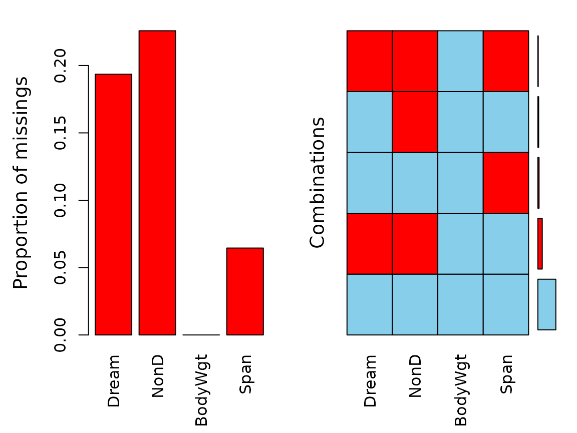

str(dataset)
#> 'data.frame':    62 obs. of  4 variables:
#>  $ Dream  : num  NA 2 NA NA 1.8 0.7 3.9 1 3.6 1.4 ...
#>  $ NonD   : num  NA 6.3 NA NA 2.1 9.1 15.8 5.2 10.9 8.3 ...
#>  $ BodyWgt: num  8.803 0 1.2194 -0.0834 7.8427 ...
#>  $ Span   : num  3.65 1.5 2.64 NA 4.23 ...

Imputation

In order to invoke the imputation methods, a formula is used to specify which variables are to be estimated and which variables should be used as regressors. We will start by imputing NonD based in BodyWgt and Span.

imp_regression <- regressionImp(NonD ~ BodyWgt + Span, dataset)
#> There still missing values in variable NonD . Probably due to missing values in the regressors.
imp_ranger <- rangerImpute(NonD ~ BodyWgt + Span, dataset)
aggr(imp_regression, delimiter = "_imp")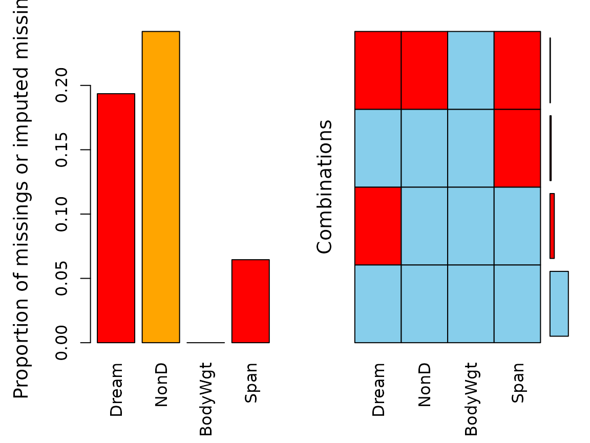

We can see that for regrssionImp() there are still missings in NonD for all observations where Span is unobserved. This is because the regression model could not be applied to those observations. The same is true for the values imputed via rangerImpute().

Diagnosing the results

As we can see in the next two plots, the correlation structure of NonD and BodyWgt is preserved by both imputation methods. In the case of regressionImp() all imputed values almost follow a straight line. This suggests that the variable Span had little to no effect on the model.

imp_regression[, c("NonD", "BodyWgt", "NonD_imp")] |> 
  marginplot(delimiter = "_imp")

For rangerImpute() on the other hand, Span played an important role in the generation of the imputed values.

imp_ranger[, c("NonD", "BodyWgt", "NonD_imp")] |> 
  marginplot(delimiter = "_imp")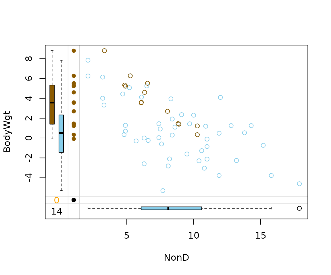

imp_ranger[, c("NonD", "Span", "NonD_imp")] |> 
  marginplot(delimiter = "_imp")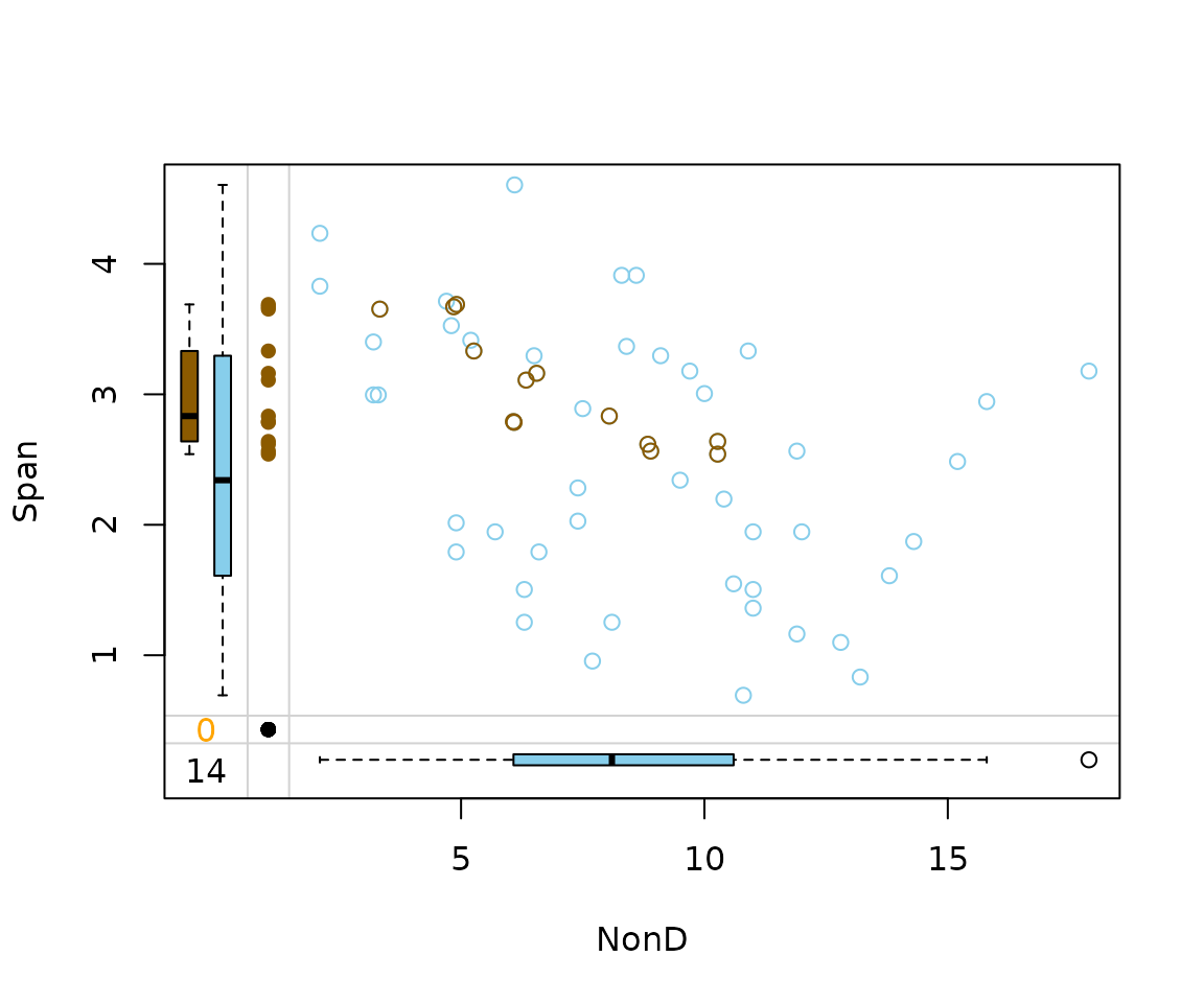

Imputing multiple variables

To impute several variables at once, the formula in rangerImpute() and regressionImp() can be specified with more than one column name in the left hand side.

imp_regression <- regressionImp(Dream + NonD ~ BodyWgt + Span, dataset)
#> There still missing values in variable Dream . Probably due to missing values in the regressors.
#> There still missing values in variable NonD . Probably due to missing values in the regressors.
imp_ranger <- rangerImpute(Dream + NonD ~ BodyWgt + Span, dataset)
aggr(imp_regression, delimiter = "_imp")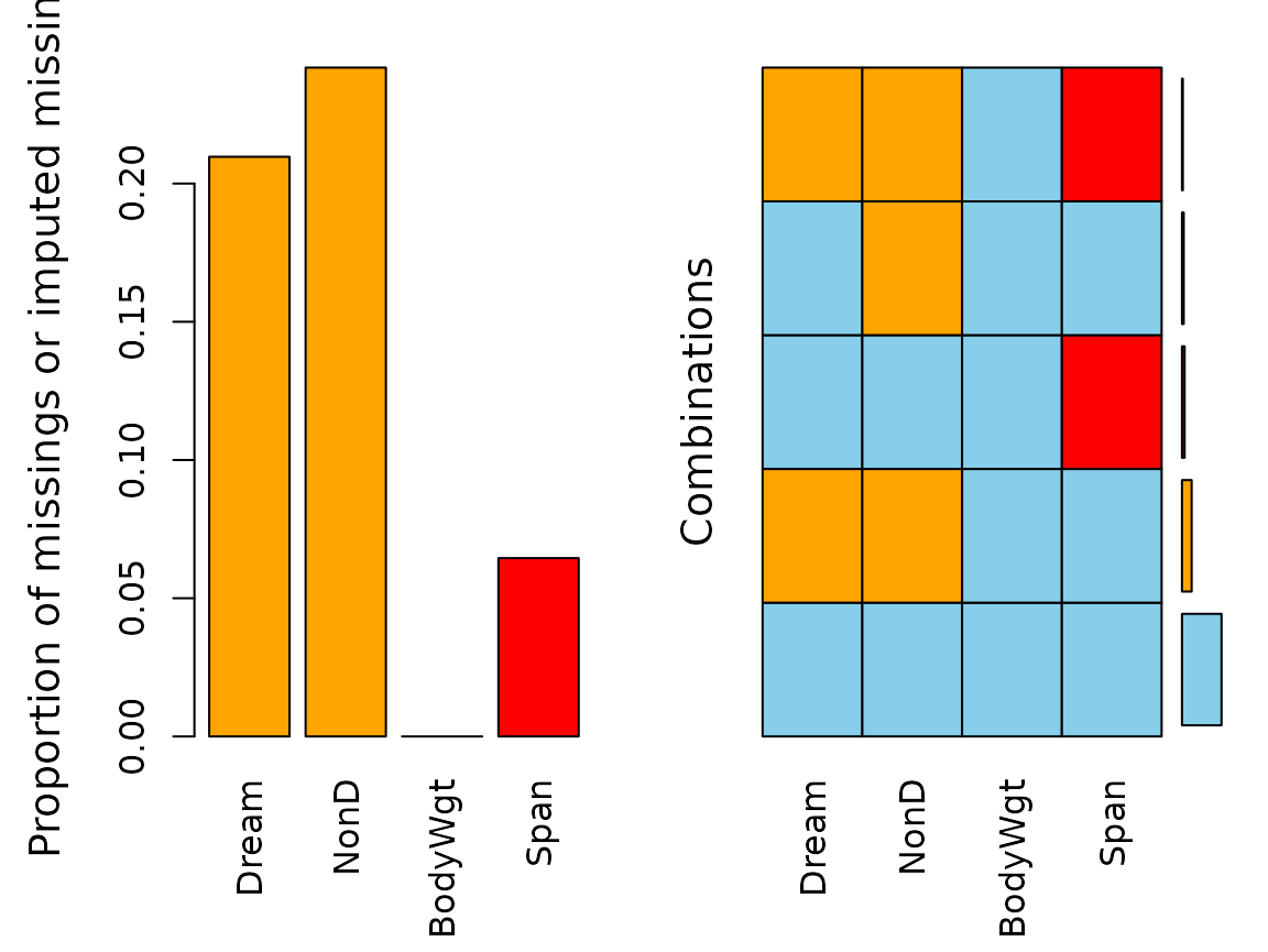

Again, there are missings left for both Dream and NonD.

Performance of method

In order to validate the performance of regressionImp() the iris dataset is used. Firstly, some values are randomly set to NA.

library(reactable)

data(iris)
df <- iris
colnames(df) <- c("S.Length","S.Width","P.Length","P.Width","Species")
# randomly produce some missing values in the data
set.seed(1)
nbr_missing <- 50
y <- data.frame(row=sample(nrow(iris),size = nbr_missing,replace = T),
                col=sample(ncol(iris)-1,size = nbr_missing,replace = T))
y<-y[!duplicated(y),]
df[as.matrix(y)]<-NA

aggr(df)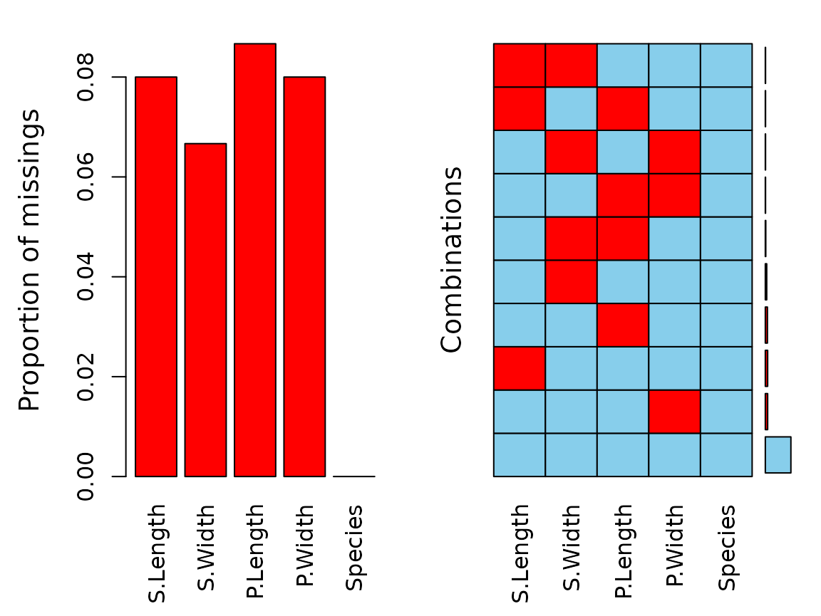

sapply(df, function(x)sum(is.na(x)))
#> S.Length  S.Width P.Length  P.Width  Species 
#>       12       10       13       12        0

We can see that there are missings in all variables and some observations reveal missing values on several points. In the next step we perform a multiple variable imputation and Species serves as a regressor.

imp_regression <- regressionImp(S.Length + S.Width + P.Length + P.Width ~ Species, df)
aggr(imp_regression, delimiter = "imp")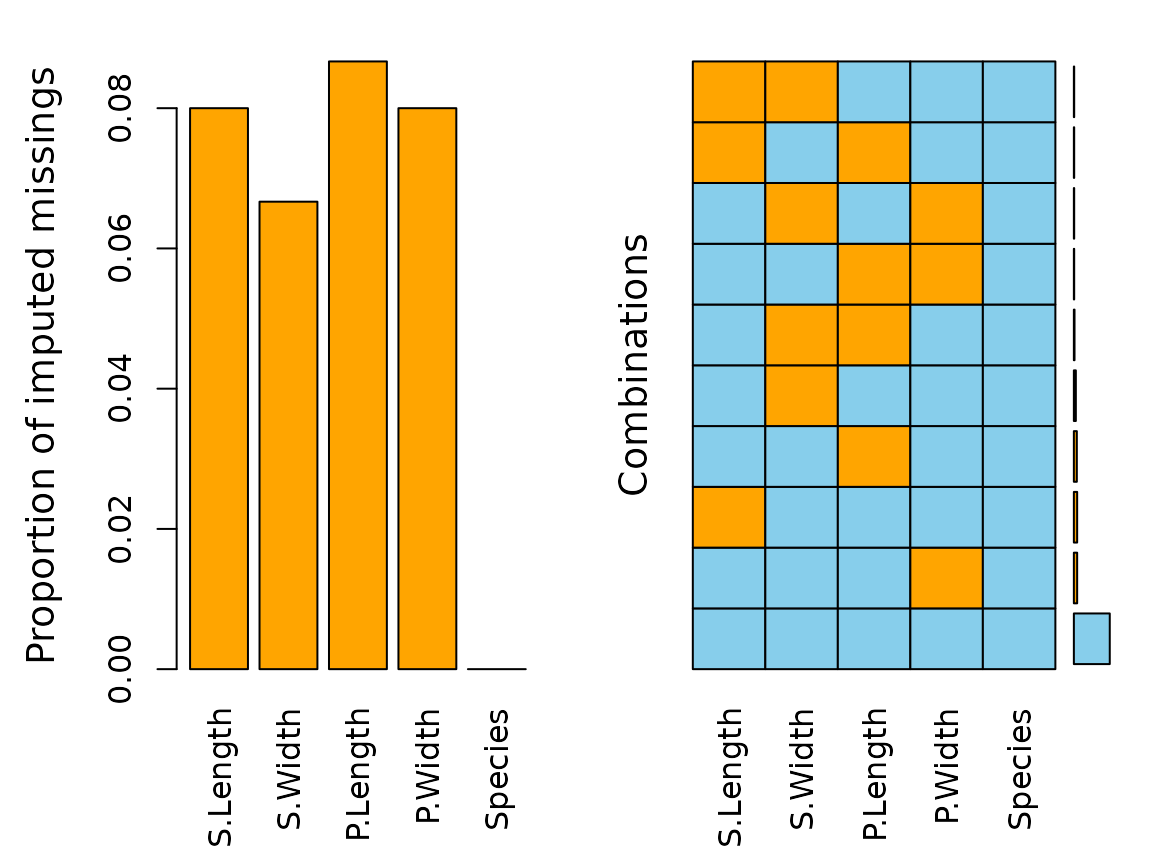

The plot indicates that all missing values have been imputed by the regressionImp() algorithm. The following table displays the rounded first five results of the imputation for all variables.