Plot surveysd-Objects — plot.surveysd • surveysd

Plot results of calc.stError()

Usage

# S3 method for class 'surveysd'
plot(
  x,
  variable = x$param$var[1],
  type = c("summary", "grouping"),
  groups = NULL,
  sd.type = c("dot", "ribbon"),
  ...
)

Arguments

x: object of class 'surveysd' output of function calc.stError
variable: Name of the variable for which standard errors have been calcualated in dat
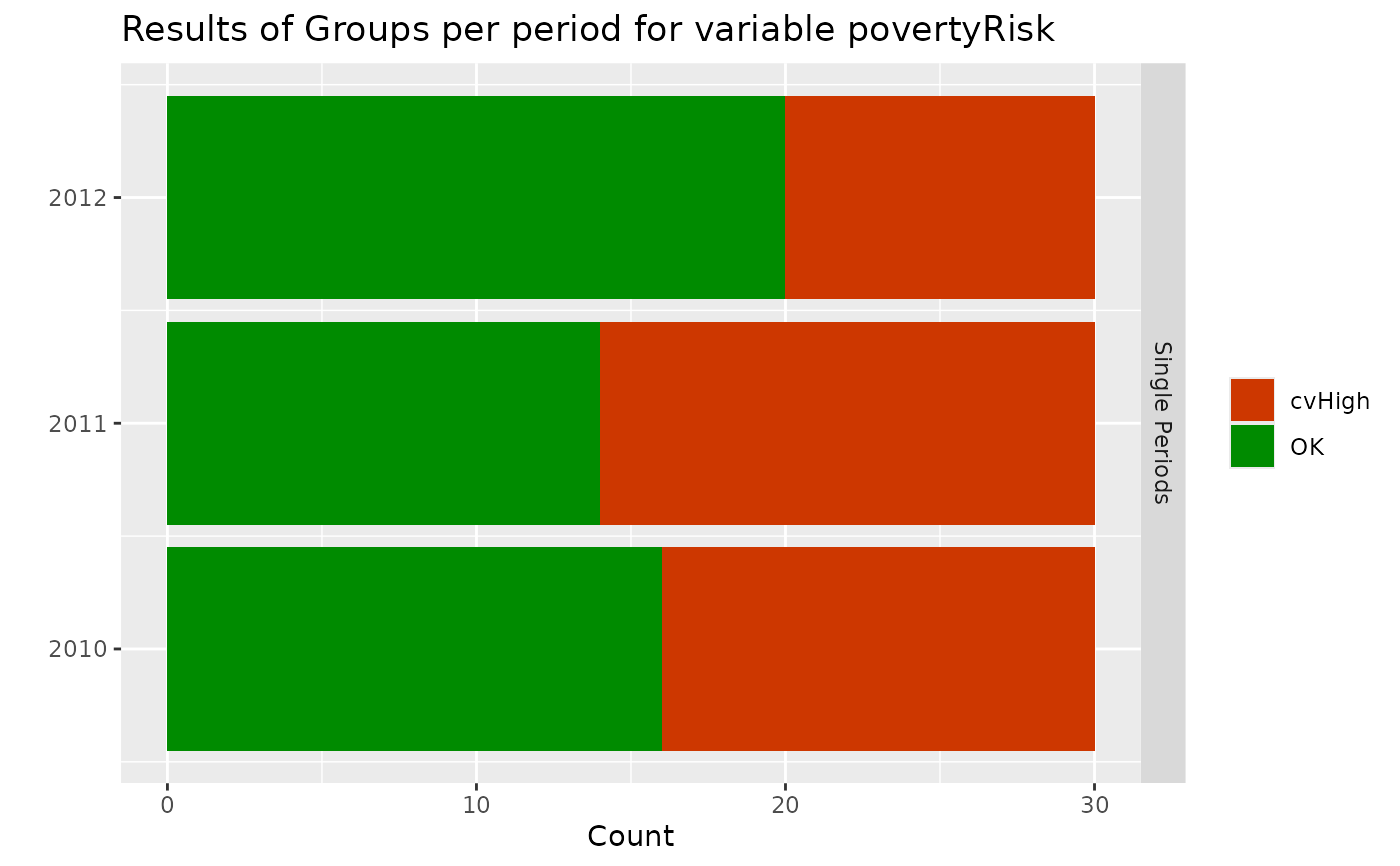
type: can bei either "summary" or "grouping", default value is "summary". For "summary" a barplot is created giving an overview of the number of estimates having the flag smallGroup, cvHigh, both or none of them. For 'grouping' results for point estimate and standard error are plotted for pre defined groups.
groups: If type='grouping' variables must be defined by which the data is grouped. Only 2 levels are supported as of right now. If only one group is defined the higher group will be the estimate over the whole period. Results are plotted for the first argument in groups as well as for the combination of groups[1] and groups[2].
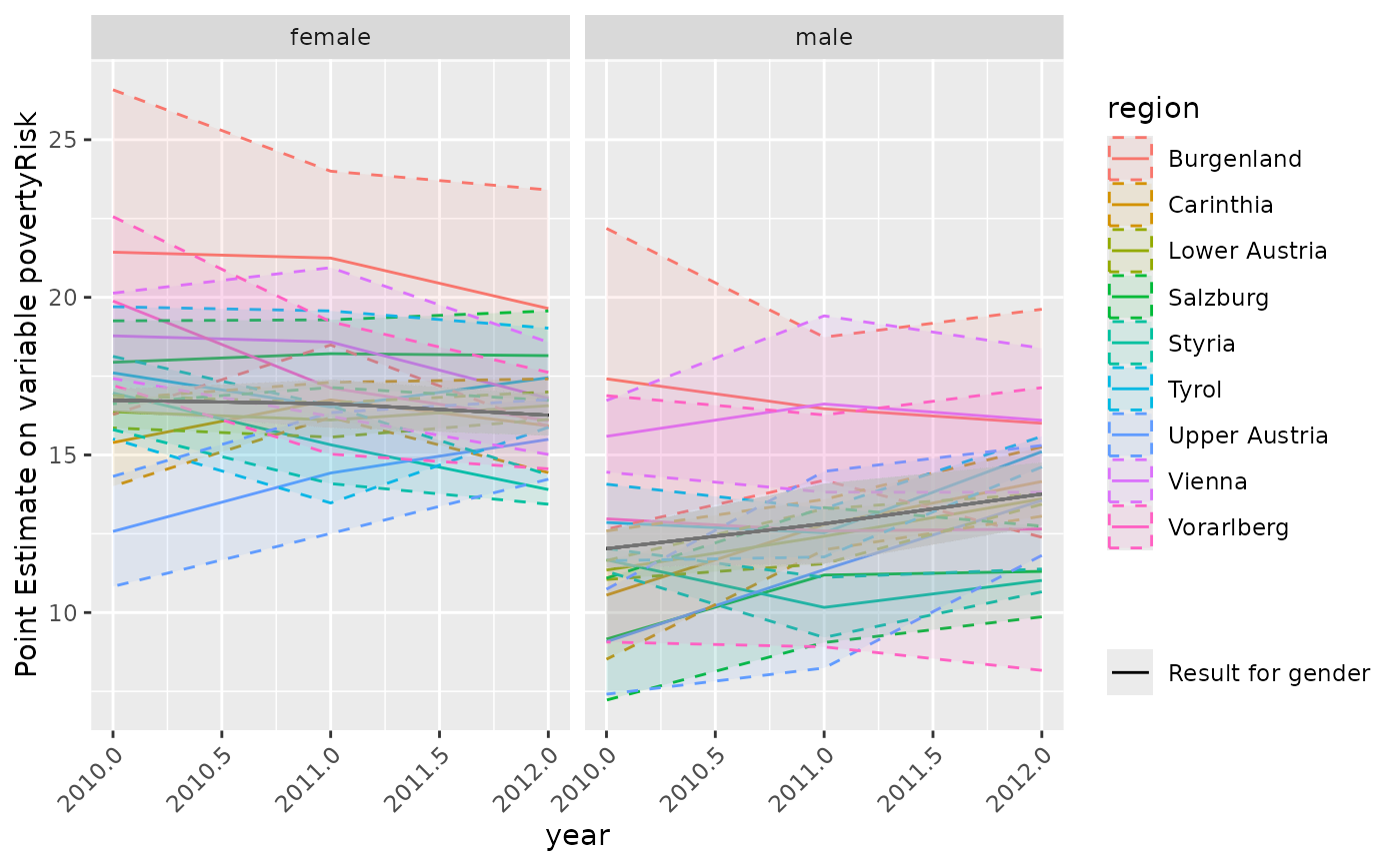
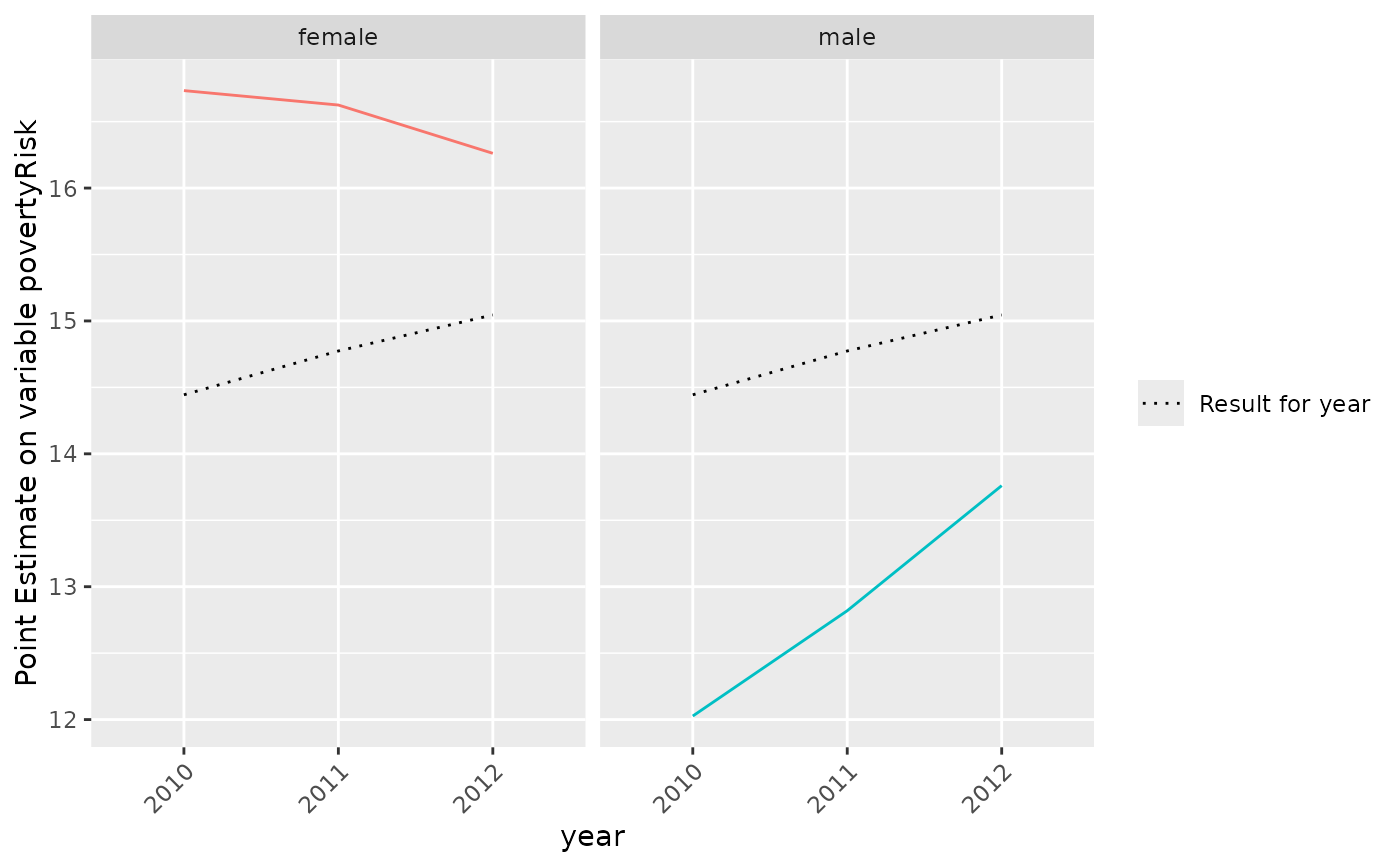
sd.type: can bei either 'ribbon' or 'dot' and is only used if type='grouping'. Default is "dot" For sd.type='dot' point estimates are plotted and flagged if the corresponding standard error and/or the standard error using the mean over k-periods exceeded the value cv.limit (see calc.stError). For sd.type='ribbon' the point estimates including ribbons, defined by point estimate +- estimated standard error are plotted. The calculated standard errors using the mean over k periods are plotted using less transparency. Results for the higher level (~groups[1]) are coloured grey.
...: additional arguments supplied to plot.

Examples


library(surveysd)

set.seed(1234)
eusilc <- demo.eusilc(n = 3, prettyNames = TRUE)

dat_boot <- draw.bootstrap(eusilc, REP = 3, hid = "hid", weights = "pWeight",
                           strata = "region", period = "year")

# calibrate weight for bootstrap replicates
dat_boot_calib <- recalib(dat_boot, conP.var = "gender", conH.var = "region")
#> Iteration stopped after 2 steps
#> Convergence reached
#> Iteration stopped after 2 steps
#> Convergence reached
#> Iteration stopped after 1 steps
#> Convergence reached

# estimate weightedRatio for povmd60 per period
group <- list("gender", "region", c("gender", "region"))
err.est <- calc.stError(dat_boot_calib, var = "povertyRisk",
                        fun = weightedRatio,
                        group = group , period.mean = NULL)


plot(err.est)


# plot results for gender
# dotted line is the result on the national level
plot(err.est, type = "grouping", groups = "gender")
#> Warning: No shared levels found between `names(values)` of the manual scale and the
#> data's shape values.



# plot results for rb090 in each db040
# with standard errors as ribbons
plot(err.est, type = "grouping", groups = c("gender", "region"), sd.type = "ribbon")