In the following example, a table will be exported from STATcube into an R session. This process involves four steps
- create a table with the STATcube GUI (table view)
- download an “API request” for the table (format:
*.json). - send the
jsonfile to the API usingsc_table(). - convert the return value into a
data.frame
It is assumed that you already provided your API key as described in the API key article.
Create a table with the STATcube GUI
Use the graphical user interface of STATcube to create a table. Visit STATcube and select a database. This will open the table view where you can create a table. See the STATcube documentation for details.
Download an API request
Choose “Open Data API Query (.json)” in the download options. This will save a json file on your local file system.
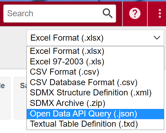
It might be the case that this download option is not listed as a download format. This means that the current user is not permitted to use the API.
Send the json to the API
Provide the path to the downloaded json file as a string in
sc_table().
This will send the json-request to the /table
endpoint of the API and return an object of class
sc_table. We will demonstrate this with an example json via
sc_example().
(json_path <- sc_example("population_timeseries.json"))
## [1] "~/R/3.6/STATcubeR/json_examples/population_timeseries.json"
my_table <- sc_table(json_path)
Printing the object my_table will summarize the data
contained in the response.
my_table#> Population at the beginning of the quarter since 2002
#>
#> Database: debevstand (STATcube)
#> Measures: Number of persons
#> Fields: Quarter <82>, Age in single years <96> <7>, Sex <2> <3>, Commune
#> <2383> (Province-District) <10>
#>
#> Request: [2022-08-29 09:52:04]
#> STATcubeR: 0.5.0.1Convert the response into a data frame
The return value of sc_table() can be converted into a
data.frame with as.data.frame().
as.data.frame(my_table)# A STATcubeR tibble: 17,220 x 5
Quarter `Age in single years <96>` `Sex <2>` Commune <2383> (Pro…¹ Numbe…²
<date> <fct> <fct> <fct> <dbl>
1 2002-01-01 Up to 14 years old male Burgenland <AT11> 21287
2 2002-01-01 Up to 14 years old male Carinthia <AT21> 47230
3 2002-01-01 Up to 14 years old male Vienna <AT13> 117920
4 2002-01-01 Up to 14 years old male Vorarlberg <AT34> 34798
5 2002-01-01 Up to 14 years old male Tyrol <AT33> 62794
6 2002-01-01 Up to 14 years old male Styria <AT22> 97538
7 2002-01-01 Up to 14 years old male Salzburg <AT32> 46955
8 2002-01-01 Up to 14 years old male Upper Austria <AT31> 127316
9 2002-01-01 Up to 14 years old male Lower Austria <AT12> 133928
10 2002-01-01 Up to 14 years old male Total 689766
# … with 17,210 more rows, and abbreviated variable names
# ¹`Commune <2383> (Province-District)`, ²`Number of persons`This will produce a data.frame, which contains a column
for each classification field of the table. Furthermore, one column will
be present for each measure. In other words, the data uses a long
format. If you prefer to use codes rather than labels, use
my_table$data instead.
my_table$data# A STATcubeR tibble: 17,220 x 5
`C-A10-0` `C-BESC51-0` `C-BESC11-0` `C-C41-2` `F-ISIS-1`
<fct> <fct> <fct> <fct> <dbl>
1 A10-20021 BESN07-1 1 B00-1 21287
2 A10-20021 BESN07-1 1 B00-2 47230
3 A10-20021 BESN07-1 1 B00-9 117920
4 A10-20021 BESN07-1 1 B00-8 34798
5 A10-20021 BESN07-1 1 B00-7 62794
6 A10-20021 BESN07-1 1 B00-6 97538
7 A10-20021 BESN07-1 1 B00-5 46955
8 A10-20021 BESN07-1 1 B00-4 127316
9 A10-20021 BESN07-1 1 B00-3 133928
10 A10-20021 BESN07-1 1 SC_TOTAL 689766
# … with 17,210 more rowsExample datasets
This article used a dataset about the austrian populatio n via
sc_example().
STATcubeR
contains more example jsons to get started. The datasets can be listed
with sc_examples_list().
sc_example("accomodation.json") %>% sc_table()#> Accomodation statistics as of 1974 according to seasons
#>
#> Database: detouextregsai (STATcube)
#> Measures: Nights spent, Arrivals
#> Fields: Season/Tourism Month <273>, Country of origin <4>, Accomodation
#> establishment <4>
#>
#> Request: [2022-08-29 09:47:07]
#> STATcubeR: 0.5.0.1
sc_example("economic_atlas.json") %>% sc_table()#> 02 Key data Federal provinces
#>
#> Database: dewatlas2 (STATcube)
#> Measures: Umemployment rate - ILO-definition, Employment rate (15 - 64 y.) -
#> ILO-definition, Overnight stays, Average duration of stay (in nights),
#> Private households, Total area (km²), Population (annual average), R&D
#> intensity (in % of GDP), Employed persons - ILO-definition, Unemployed -
#> ILO-definition, … (38 more)
#> Fields: Year (starting 1995) <28>, Federal provices <11>
#>
#> Request: [2022-09-21 11:18:57]
#> STATcubeR: 0.5.0.1
sc_example("foreign_trade.json") %>% sc_table()#> Trade by commodity (CPA) and activity sector (NACE)
#>
#> Database: denatec06 (STATcube)
#> Measures: Import, number of enterprises, Import, value in Euro, Export,
#> number of enterprises, Export, value in Euro
#> Fields: Commodities (CPA) <4>, Reference year <13>, Activity Sector (NACE)
#> [partly ABO] <4>
#>
#> Request: [2022-08-30 19:08:33]
#> STATcubeR: 0.5.0.1
sc_example("gross_regional_product.json") %>% sc_table()#> Gross regional product by ESA 1995, NUTS2+NUTS3 - finished time
#> series
#>
#> Database: devgrrgr004 (STATcube)
#> Measures: Gross regional product; current prices in million Euro, Gross
#> regional product per inhabitant, Gross regional product per person
#> employed
#> Fields: NUTS-3 <11>, Time <13>
#>
#> Request: [2022-08-30 19:06:56]
#> STATcubeR: 0.5.0.1
sc_example("labor_force_survey.json") %>% sc_table()#> Working hours (Labour Force Survey)
#>
#> Database: deake005 (STATcube)
#> Measures: Average hours actually worked per week, Average hours usually
#> worked per week
#> Fields: Time section <8>, Gender <3>, Highest level of training completed
#> (national classification) <6>, Province (NUTS 2 unit) <10>
#>
#> Request: [2022-08-31 12:48:22]
#> STATcubeR: 0.5.0.1
sc_example("agriculture_prices.json") %>% sc_table()#> EAA01_Economic accounts for agriculture at current prices in million
#> euros
#>
#> Database: delgr001 (STATcube)
#> Measures: Values (for output items and value added: values at basic prices),
#> Taxes on products (for output items), Values at producer prices (for
#> output items), Subsidies on products (for output items)
#> Fields: Year <28>, Item <6>
#>
#> Request: [2022-09-21 11:19:01]
#> STATcubeR: 0.5.0.1
sc_example("economic_trend_monitor.json") %>% sc_table()#> Economic Trend Monitor
#>
#> Database: dekonjunkturmonitor (STATcube)
#> Measures: Production Index Industry (wd; 2015=100), Technical total
#> production Industry (in 1.000 €), Turnover Index Industry (2015=100),
#> Turnover Industry (in 1.000 €), Index of new orders Industry (2015=100),
#> Index of persons employed Industry (2015=100), Persons employed Industry,
#> Productivity Index Industry per employee (2015=100), Productivity Index
#> Industry per hours worked (2015=100), Industrial Output Price Index
#> (2021=100), … (53 more)
#> Fields: reporting period <165>, value indication <2>
#>
#> Request: [2022-09-21 11:19:05]
#> STATcubeR: 0.5.0.1Choosing the Language
The language which is used for labelling can be changed via the
language parameter of sc_table().
sc_example("accomodation.json") %>% sc_table("de")#> Nächtigungsstatistik ab 2000 nach Regionen und Saison
#>
#> Database: detouextregsai (STATcube)
#> Measures: Übernachtungen, Ankünfte
#> Fields: Saison/Tourismusmonat <273>, Herkunftsland <4>, Beherbergungsbetrieb
#> <4>
#>
#> Request: [2022-08-29 09:48:09]
#> STATcubeR: 0.5.0.1
sc_example("economic_atlas.json") %>% sc_table("de")#> 02 Eckdaten Bundesländer
#>
#> Database: dewatlas2 (STATcube)
#> Measures: Arbeitslosenquote - ILO, Erwerbstätigenquote (15-64 J.) - ILO,
#> Nächtigungen, Durchschnittliche Aufenthaltsdauer in Tagen,
#> Privathaushalte, Fläche (km²), Wohnbevölkerung im Jahresdurchschnitt,
#> Forschungsquote (in % des BIP), Erwerbstätige - ILO, Arbeitslose - ILO, …
#> (38 more)
#> Fields: Jahr (ab 1995) <28>, Bundesland <11>
#>
#> Request: [2022-09-30 14:49:44]
#> STATcubeR: 0.5.0.1
sc_example("foreign_trade.json") %>% sc_table("de")#> Außenhandel nach Gütern (CPA) und Wirtschaftszweig (NACE)
#>
#> Database: denatec06 (STATcube)
#> Measures: Import; Anzahl der Unternehmen, Import, Wert in Euro, Export;
#> Anzahl der Unternehmen, Export, Wert in Euro
#> Fields: Güter (CPA) <4>, Berichtsjahr <13>, Wirtschaftszweig (NACE) [teilw.
#> ABO] <4>
#>
#> Request: [2022-09-30 14:49:50]
#> STATcubeR: 0.5.0.1
sc_example("gross_regional_product.json") %>% sc_table("de")#> Bruttoregionalprodukt nach ESVG 1995, NUTS2+NUTS3 - abgeschlossene
#> Zeitreihe
#>
#> Database: devgrrgr004 (STATcube)
#> Measures: Bruttoregionalprodukt nominell in Mio.Euro, Bruttoregionalprodukt
#> je Einwohner, Bruttoregionalprodukt je Erwerbstätigem
#> Fields: NUTS-3 <11>, Zeit <13>
#>
#> Request: [2022-09-30 14:49:53]
#> STATcubeR: 0.5.0.1
sc_example("labor_force_survey.json") %>% sc_table("de")#> Mikrozensus-Arbeitskräfteerhebung Arbeitsstunden
#>
#> Database: deake005 (STATcube)
#> Measures: Durchschn. tatsächlich geleistete Arbeitsstunden pro Woche,
#> Durchschn. Normalarbeitsstunden pro Woche
#> Fields: Zeit <8>, Geschlecht <3>, Höchste abgeschlossene Schulbildung -
#> nationale Gliederung <6>, Bundesland (NUTS 2-Einheit) <10>
#>
#> Request: [2022-09-30 14:50:04]
#> STATcubeR: 0.5.0.1
sc_example("agriculture_prices.json") %>% sc_table("de")#> LGR01_Landwirtschaftliche Gesamtrechnung zu laufenden Preisen in
#> Millionen Euro
#>
#> Database: delgr001 (STATcube)
#> Measures: Werte (für Positionen der Produktion sowie Wertschöpfung: Werte zu
#> Herstellungspreisen), Gütersteuern (für Positionen der Produktion), Werte
#> zu Erzeugerpreisen (für Positionen der Produktion), Gütersubventionen (für
#> Positionen der Produktion)
#> Fields: Jahr <28>, Position <6>
#>
#> Request: [2022-09-26 14:41:37]
#> STATcubeR: 0.5.0.1
sc_example("economic_trend_monitor.json") %>% sc_table("de")#> Konjunkturmonitor
#>
#> Database: dekonjunkturmonitor (STATcube)
#> Measures: Produktionsindex Industrie (at; 2015=100), Technische
#> Gesamtproduktion Industrie in Tsd. € (KJE), Umsatzindex Industrie
#> (2015=100), Umsatz Industrie inTsd.€ (KJE), Auftragseingangsindex
#> Industrie (2015=100), Beschäftigtenindex Industrie (2015=100),
#> Beschäftigte Industrie gesamt (KJE), Produktivitätsindex Industrie je
#> unselbständig Beschäftigtem (2015=100), Produktivitätsindex Industrie je
#> geleisteter Arbeitsstunde (2015=100), Erzeugerpreisindex für den
#> Produzierenden Bereich (2021=100; NACE B-E), … (53 more)
#> Fields: Berichtszeitraum <165>, Wertangabe <2>
#>
#> Request: [2022-09-30 14:50:08]
#> STATcubeR: 0.5.0.1Further reading
- Functionalities of the returned object are explained in the STATcubeR data article.
-
sc_tabulate()provides a more flixble way of turning STATcube tables intodata.frames. See the tabulation article for more details. - The saved tables article shows an alternative way of importing tables.
- If you are interested in other API endpoints, see the schema article ot the other API endpoints article